Lateral Compression of Thin-Walled c/s #

The study of lateral compression of thin-walled cross-sections is crucial in understanding the mechanical behavior and structural integrity of materials under load. This type of deformation is particularly relevant in applications such as aerospace, automotive, and civil engineering, where tubes and other hollow sections are commonly used. The lateral compression test, or ring compression test, provides valuable insights into material properties and failure mechanisms.

In a lateral compression experiment also known as ring compression, a tube is placed horizontally between two fixed rigid flat plates as shown in the illustration. The setup ensures that the tube's rib is balanced between the plates. The tube is then subjected to a quasi-static load, and the corresponding load-displacement responses are recorded as depicted in the ideal Load-Displacement plots. This setup allows for the controlled application of load and precise measurement of the tube's response. The lateral compressed tube obtains a shape of similar to horseback saddle when view from the compressed direction.

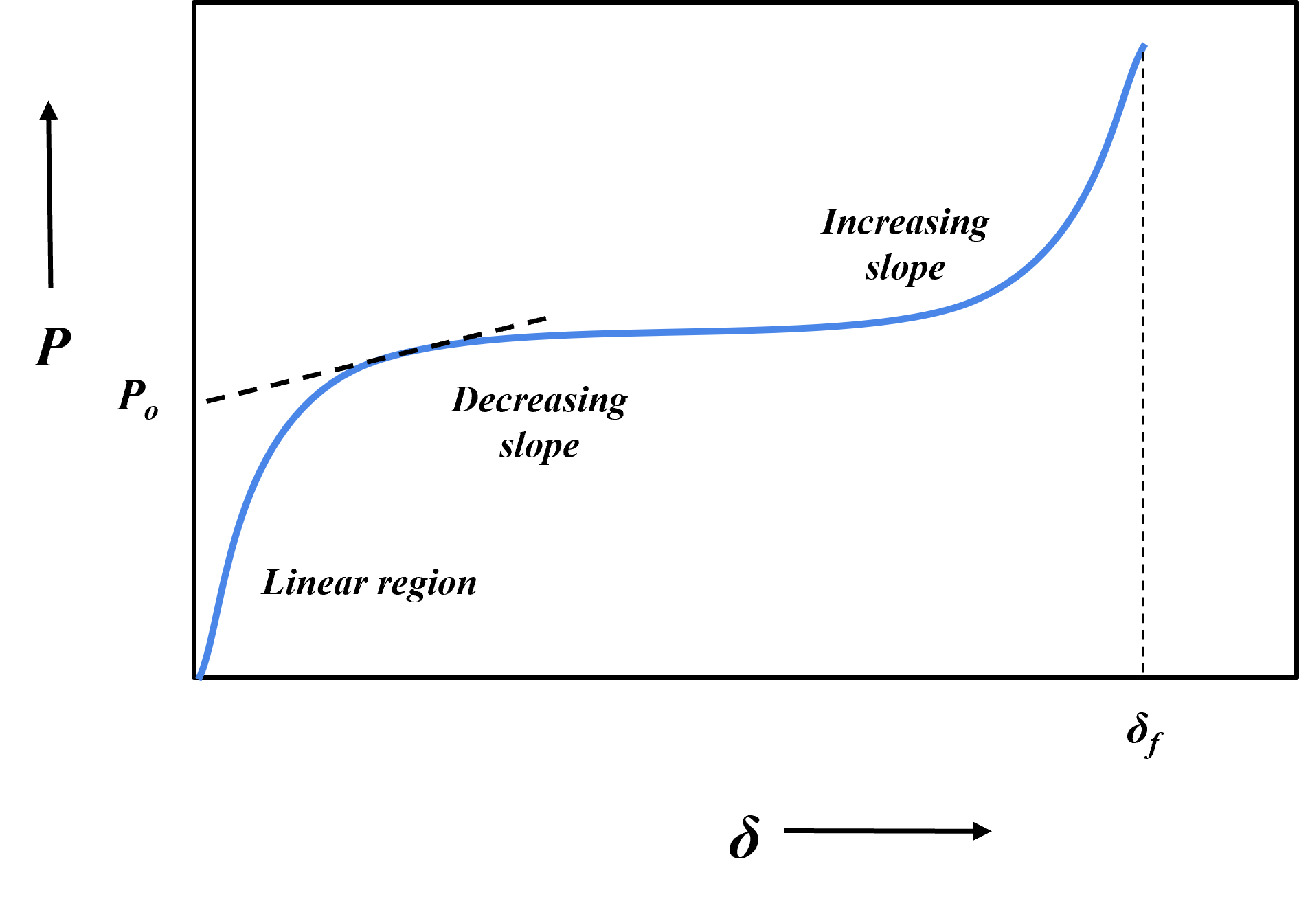
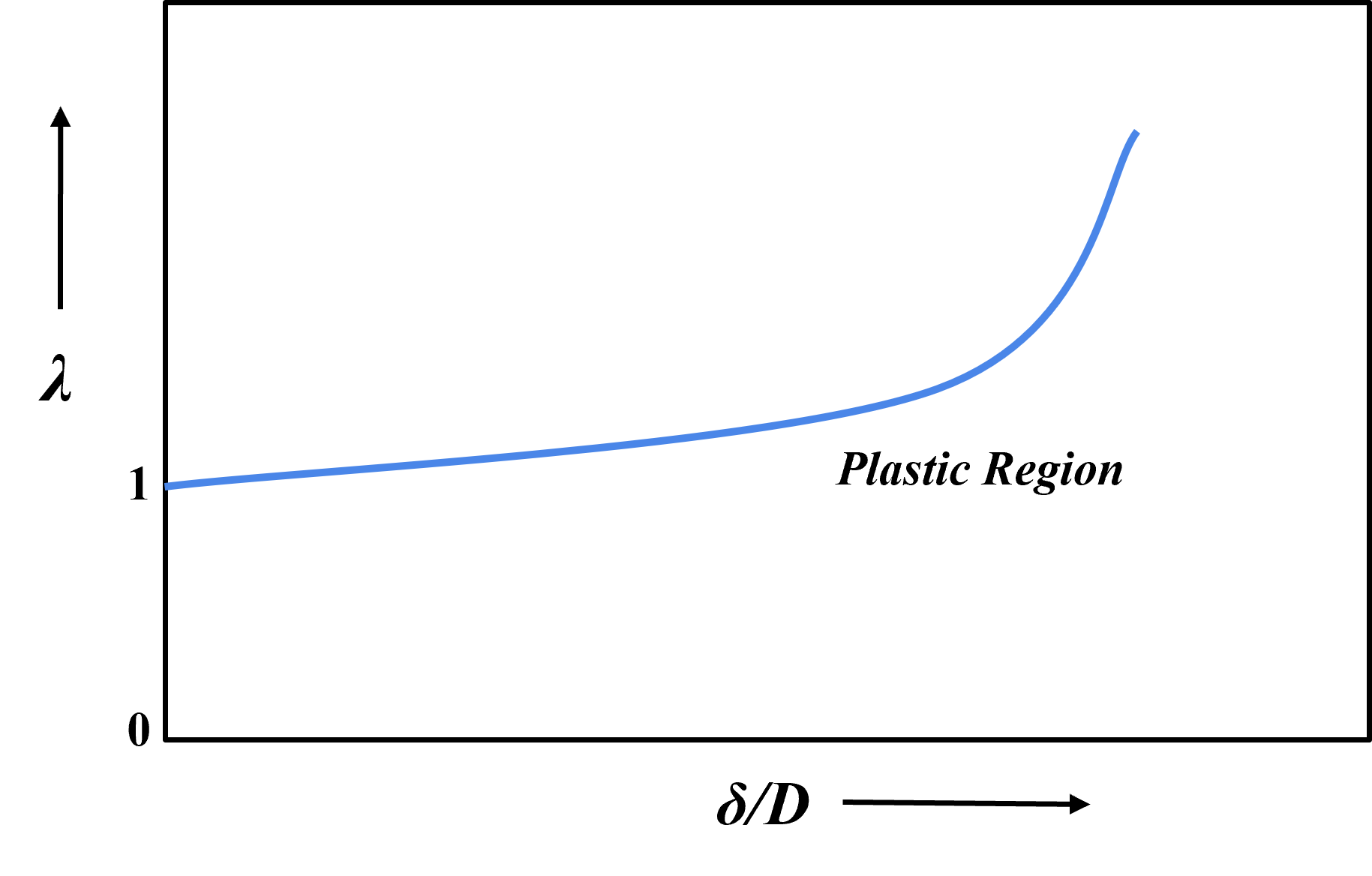
The corresponding load displacement characteristic obtained from the lateral compression. The tube is loaded in quasi-static condition, that is loading is applied slowly at a constant deformation rate. The ideal load-displacement curve depicts the linear elastic region, the constant yield part of the curve. And once plastic deformation is occured, the slope increases. The same is represented with a zoomed part of the curve in the adjacent plot. The Load-Displacement curve can be divided into three different phases:

• Elastic Loading Phase: Initially, the load-displacement relationship is linear, indicating elastic behavior. In this region, the tube deforms elastically and returns to its original shape upon unloading.
• Yielding Phase: As the load increases, the tube reaches its yield point, where plastic deformation begins. This phase is characterized by a stabilization of the load, as the material undergoes permanent deformation.
• Plastic Deformation Phase: Beyond the yield point, the tube undergoes plastic deformation. This phase is represented by an increasing slope on the load-displacement curve, indicating that the material continues to deform plastically under the applied load.

---

Experiment #

The method of ring compression test of tubes is useful in determining material properties such as yield strength and modulus of elasticity. A relation between yield stress and limit load were plastic deformation is initiated for tube under lateral compression of tube is given as:

\[ \sigma_y = \alpha P_l r_o / lt^2 \]

the conditions given for selecting the value of α are

\[ \alpha=1.0, l \le xt (1 \le x \le 5) \] \[\alpha=0.866, l \ge 2r_o \]

The modulus of elasticity E of the tube material can be derived based on elastic load and elastic deflection and this was proposed by DeRuntz and Hodge and is given as:

\[ E = \frac{12P_e (r_o)^3 \beta}{\delta_e t^3 l} (\frac{\pi}{4} - \frac{2}{\pi})\]

Here, \( \beta = 1 \) for plane stress and \( \beta = 1 – \nu^2 \) plane strain

The experiment were conducted for aluminium 6063 tube specimen of dimensions 50mm length and 50mm diameter and 1.6mm thickness was subjected to lateral compression. The tube was tested under quasi-static conditions at a constant deformation rate of 4mm/min. The stages of compression of the tubes were captured to understand the deformation under circumferential load. Simultaneously, the load-displacement response was recorded for the same.

In the Load-Displacement response is recorded based on the change in pressure per the circumferential area to the change in displacement in the lateral direction. To find the collapse load or plastic load \(P_o \), a line is drawn at the conjunction of the elastic and plastic region and dragged until the y-coordinate value is determined. The value determined for \(P_o \) for this experiment is 0.94kN.

With the attained values from the experiment and the pre-loaded or determined values for the material properties, the following is calculated as follows.
For the calculation of Yield Stress, the data is as follows:
Pl=0.94kN; ro=25mm; t=1.6mm; l=50mm \[\sigma_y = \frac{1* 0.94 * 10^3 *25}{1.6^2 * 50} = 183.6MPa\] For the calculation of the Youngs Modulus, the data is as follows:
Pe=0.8kN; ro=25mm; t=1.6mm; l=50mm; β=1mm (Plane stress condition); δe=1.6mm \[ E = \frac{12 * 0.8 * 10^3 * 25^3 * 1}{1.6 * 1.6^3 * 50} (\frac{\pi}{4} - \frac{2}{\pi}) = 68.206GPa\]

---

Theoretical Study #

To derive the theoretical load-deflection curve for lateral compression of thin-walled tubes, a dimensionless parameter namely mR is derived and is given as, \[mR =\left(\frac{6 \sigma_o R}{E_p t}\right)^{1/2} \] Where σo is the yield stress and is obtained as dependency on the collapse load Po and is given as: \[ P_o = \sigma_o t^2 / R\] rearranged to obtain the yield stress σo, and is given as: \[\sigma_o = \frac{\alpha P_o R}{t^2} \frac{1}{l}\] Here α =1, if rings (L>T)
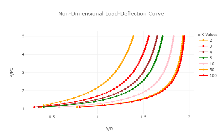
Ep is obtained as the average hardening modulus and is deduced based on the best fit that is obtained for the mR values mapped on a load-displacement plot. For different input values of the parameter mR, the theoretical load-deflection was derived, plotted and observed.

In the figure representing the non-dimensional entity \(mR\). These curves can be used reverse to plot the Load-Displacement reponse with the value of mR assumed. The best fit and value for \(mR\) is chosen based on comparison with the non-dimensional experimental load-displacement curve. With this the obtained value of mR, consequently the average hardening modulus Ep can be obtained.

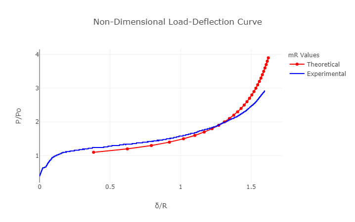
For futher analysis and calculations, the experimental Load-Displacement curve is converted to Non-Dimensional curve. From the Load-Displacement curve, the 'x' and 'y' axes data are converted to non-dimensional entities. The data from the 'x' column i.e. displacement is divided by the radius of the sample tube. In this case of experiment, the tube radius is measured to be 25mm. Similarly, the data from the 'y' column i.e. Load is divided by the collapse load (Po). Hence the resulting plot obtain is non-dimensional, i.e., P/Po v/s δ/R.

In respone to the mR value, the theortical and experimental curves are both plotted together on a non-dimensional plot. The mR value is changed so that the theoretical and experimental curves find a best fit. In the plot depicted below, the closest fit was found for a mR value of 4. This values can be further used for material characterisation.

Using the equation of mR for the obtained values of 4, the hardening modulus Ep is attained for the following inputs,
\(mR=4; \sigma_o=183.6MPa; R=25mm; t=1.6mm \) \[4=[(6*183.6*25)/(E_p * 1.6)]^{1/2}\] \[E_p = 1.075GPa\] The hardening modulus \(Ep\) for the aluminium 6063 tube is calculated as \(1.075GPa\).

---

This calculator generates a theoretical load-deflection curve for the lateral compression of thin-walled tubes. It allows users to input specific parameters related to the experiment and visualize the resulting curve on a plot.
User Inputs: \(mr, \lambda_{min}, \lambda_{max}\)
This checkbox allows users to decide whether to retain the existing plot and add new curves to it or to replace the existing plot with a new one. If checked, new curves will be added to the existing plot with different colors. The resulting plot will show the load-deflection curve, with different colors representing different calculations. The legend on the plot will list the mR values used for each curve.

---

References #

• S.R. Reid, T.Yella Reddy. (1978) Effect of strain hardening on the lateral compression of tubes between rigid plates. Int. J. Solids and Structures
• T. Yella Reddy And S. R. Reid. (1979) Lateral Compression Of Tubes And Tube-Systems With Side Constraints. Int. J. Mech. Sci.
• T. Yella Reddy, S. R. Reid. (1979) On obtaining material properties from the ring compression test. Nuclear Engineering and Design