01Overview
The Split Hopkinson Pressure Bar (SHPB), or Kolsky bar, measures how materials behave when they are deformed very quickly: the conditions of a crash, a blast or a ballistic impact. A short specimen sits between two long elastic bars. A striker hits the first bar, a stress pulse runs down it into the specimen, and strain gauges on both bars record what goes in, what is reflected and what passes through. From those three signals, one-dimensional wave theory gives the specimen's stress, strain and strain rate over time.
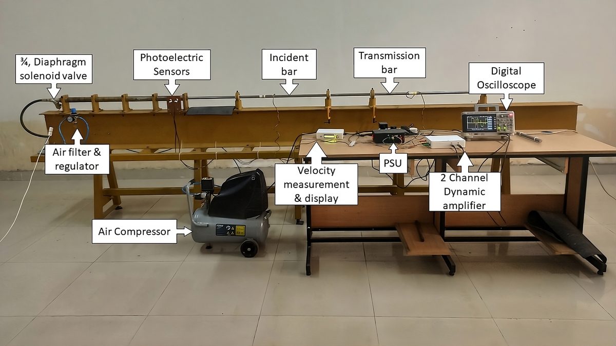
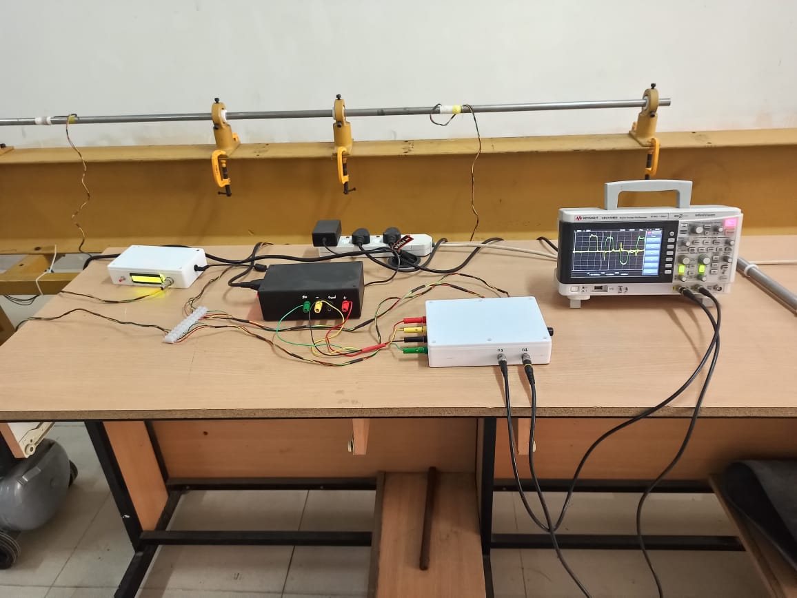
I led the project end to end: design and CAD of the frame and bars, manufacture, the compressed-air striker launcher, an infrared velocity gate, a two-channel strain-gauge amplifier, testing, and the MATLAB and Python software that reduces the data.
02The method
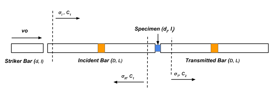
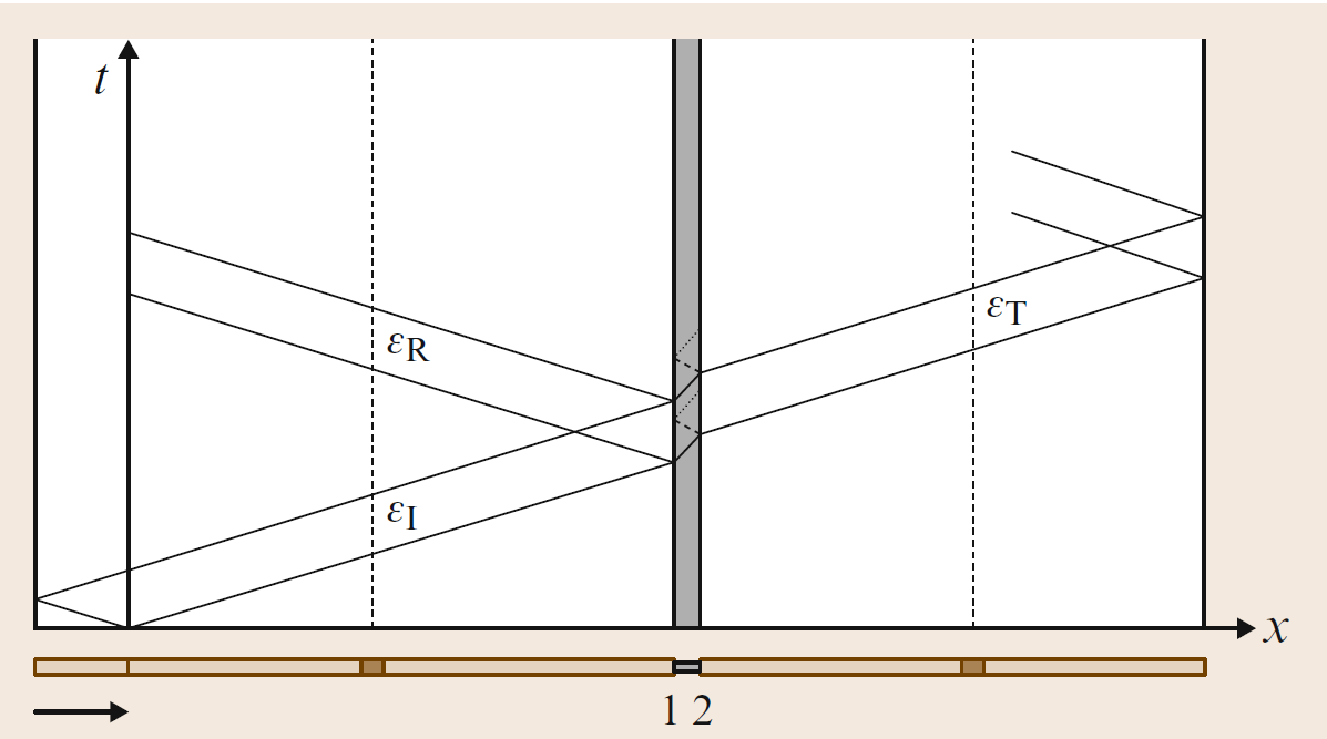
The input (incident) and output (transmitted) bars stay elastic throughout the test; only the specimen deforms plastically. The bars are high-strength steel, and the striker is the same material as the bars. When the striker hits the input bar, a compressive pulse travels to the specimen. Part of it is reflected back into the input bar and part is transmitted through the specimen into the output bar. The gauges are placed so the incident and reflected pulses do not overlap.
- Incident pulse: generated by the striker impact.
- Reflected pulse: from the input bar / specimen interface; it carries the specimen's strain rate.
- Transmitted pulse: through the specimen into the output bar; it carries the specimen's stress.
The SHPB covers the high strain-rate range, 10² to 10⁴ s⁻¹, above what servo-hydraulic machines and drop towers can reach and below plate-impact tests.
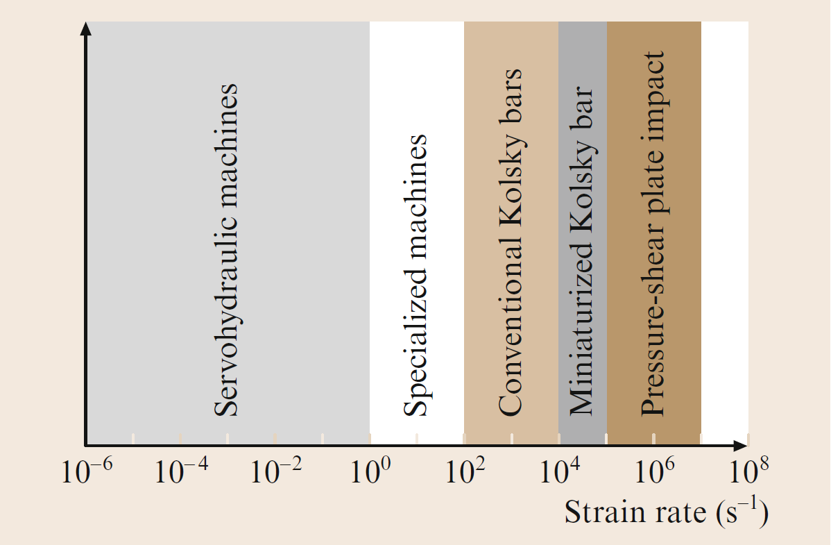
Where it is used
- Dynamic strength of metals, ceramics, composites and polymers for armour, pipelines, pressure vessels and offshore structures.
- Crashworthiness of aerospace and automotive materials, and the impact response of protective gear.
- Effects of temperature, strain rate, loading history and microstructure on flow stress.
03Design of the bar
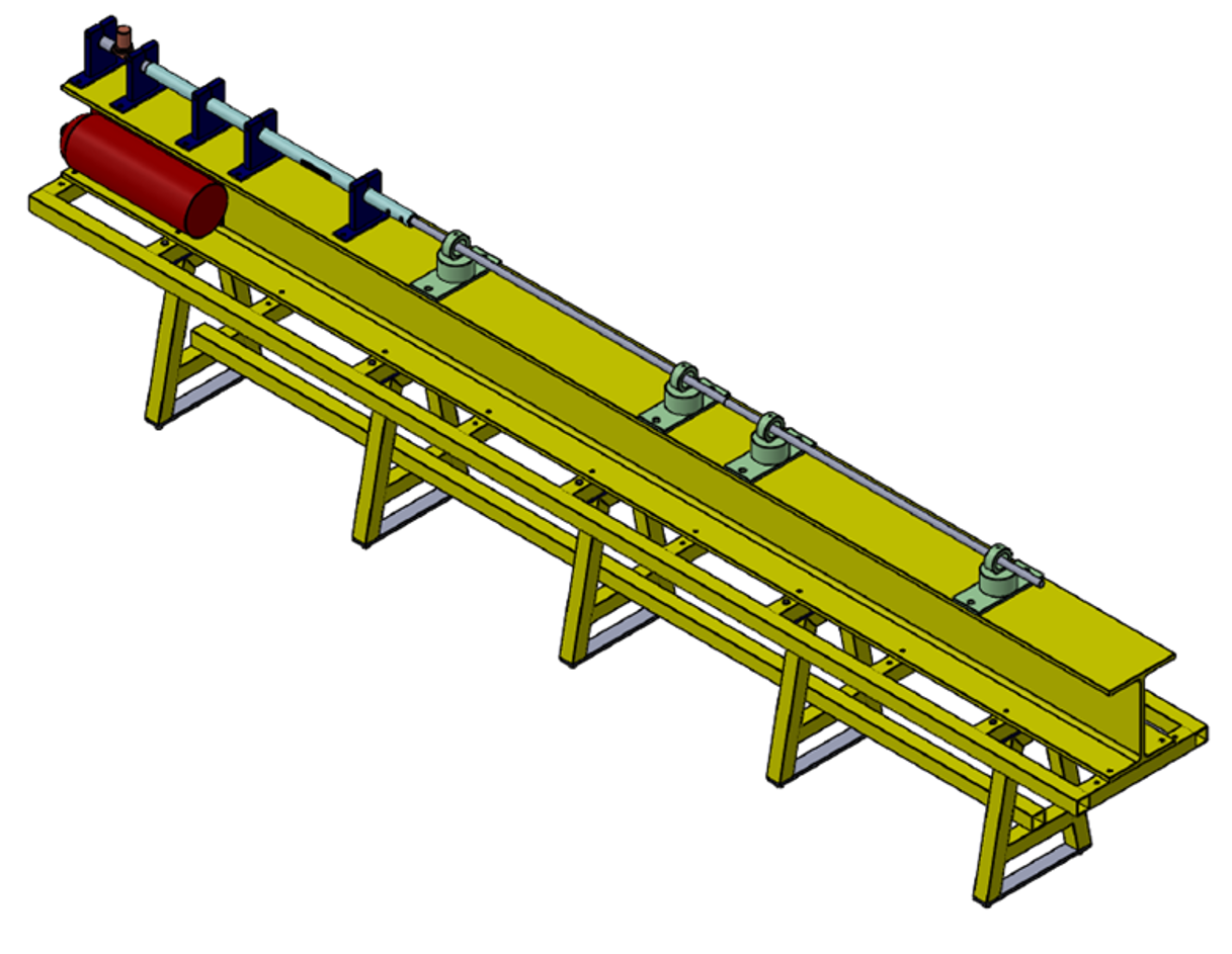
The whole apparatus sits on an I-beam, the backbone that carries the gas gun and the holders for the incident and transmitted bars. The holders are machined so the gun barrel and both bars share one centreline. A 4 m ladder frame raises the beam to working height, five A-frames stiffen the structure, and levelling screws on every leg let the line be aligned precisely.
Design rules
- Ratios: bar length to diameter L/D ≈ 100; bar to specimen diameter D/d₀ = 2–4; specimen length to diameter l₀/d₀ = 0.6–1.
- Bar length: long enough that incident and reflected pulses do not overlap at the gauge.
- Alignment: bars and specimen on one axis, to keep the stress uniaxial and the tests repeatable.
- Specimen: flat, parallel, lubricated faces to limit friction and stress concentrations.
- Acquisition: high-speed, synchronised recording of both bars and the striker velocity.
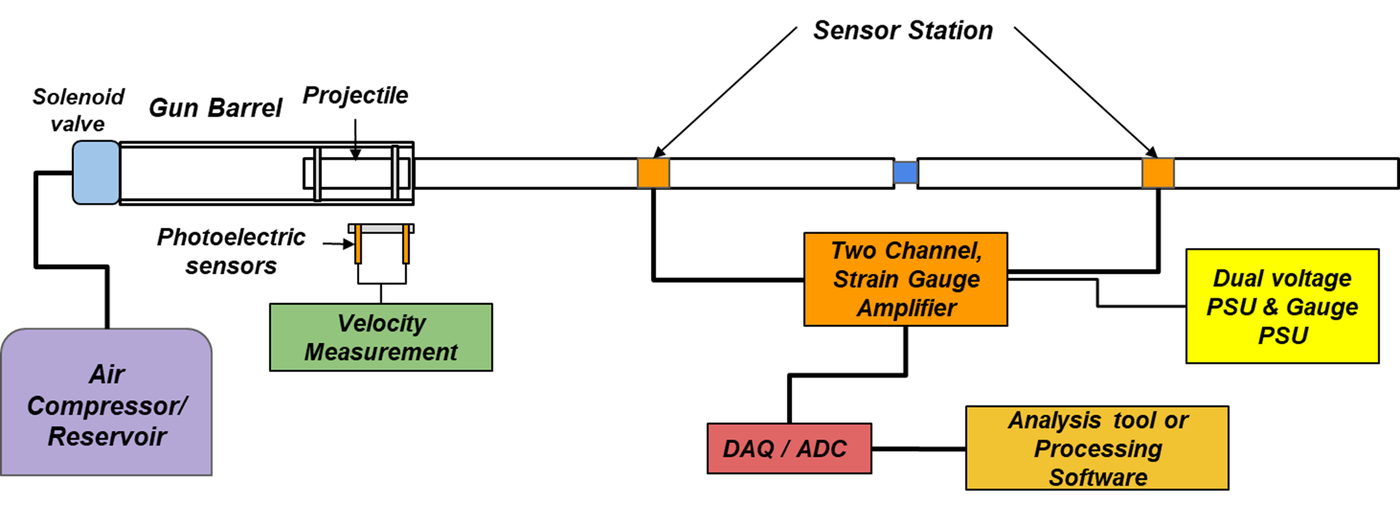
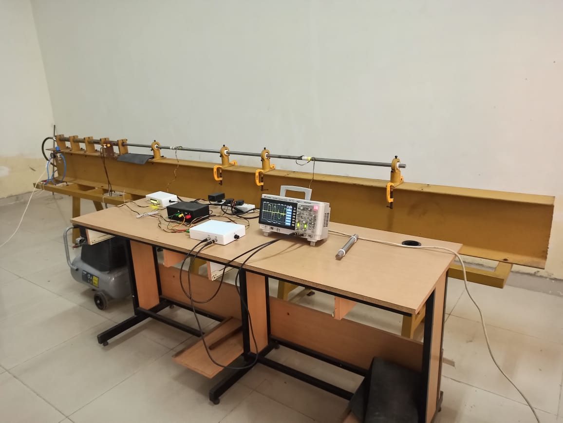
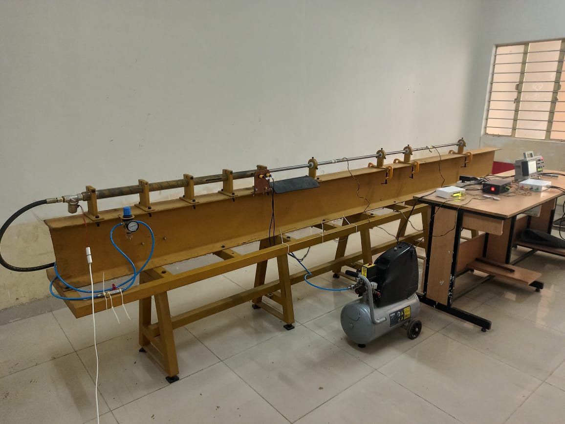
Drawings: assembly (PDF) · parts (PDF).
04Striker launch system
A compressed-air gas gun fires the striker into the incident bar. The launch pressure sets the striker speed, and so the energy of the impact and the strain rate in the specimen.
- An air compressor fills a storage cylinder.
- A flow controller, filter and ball valve feed a reservoir tank through a non-return valve; the reservoir is charged to the exact pressure for the speed wanted.
- A 3/8 in, 180 bar hydraulic hose links the reservoir to the barrel.
- A 3/4 in normally closed diaphragm solenoid valve (220 V AC) sits at the barrel; pressing the button opens it and the air drives the striker down the barrel.
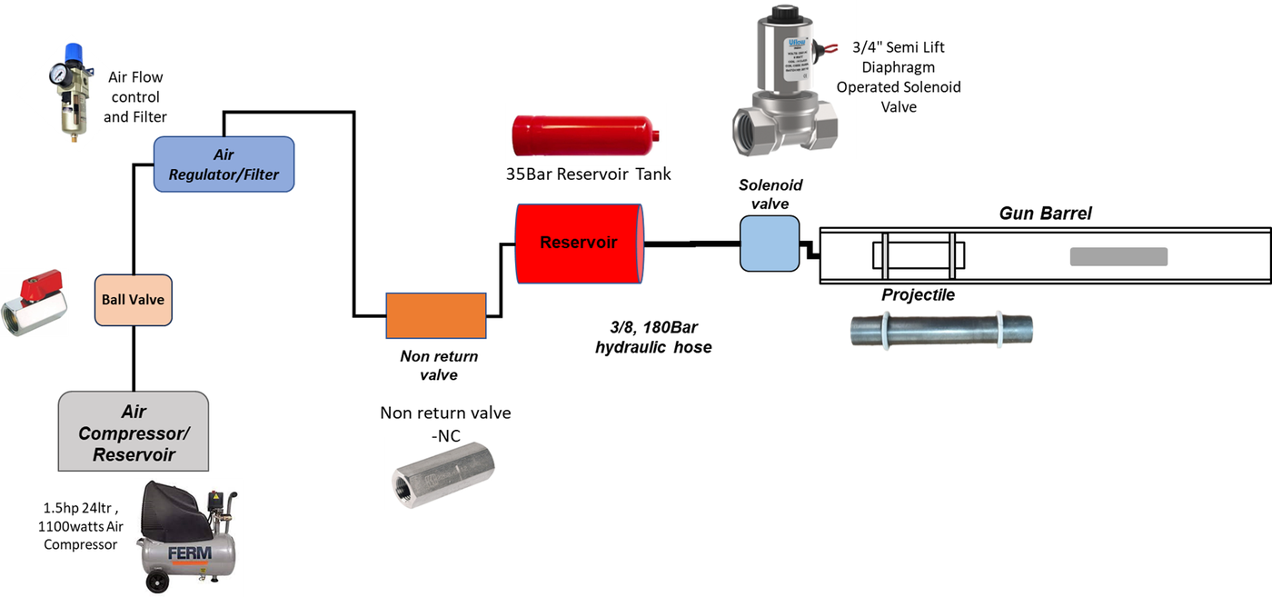
The launch velocity follows from the reservoir pressure , the barrel area , the striker mass and its travel in the barrel (an upper bound, since it ignores friction and expansion of the air):
05Velocity measurement
Two infrared sensors 50 mm apart sit at the barrel exit. An Arduino Uno records the moments each beam is broken, in microseconds, and a 16×2 LCD shows the transit time and the striker velocity:
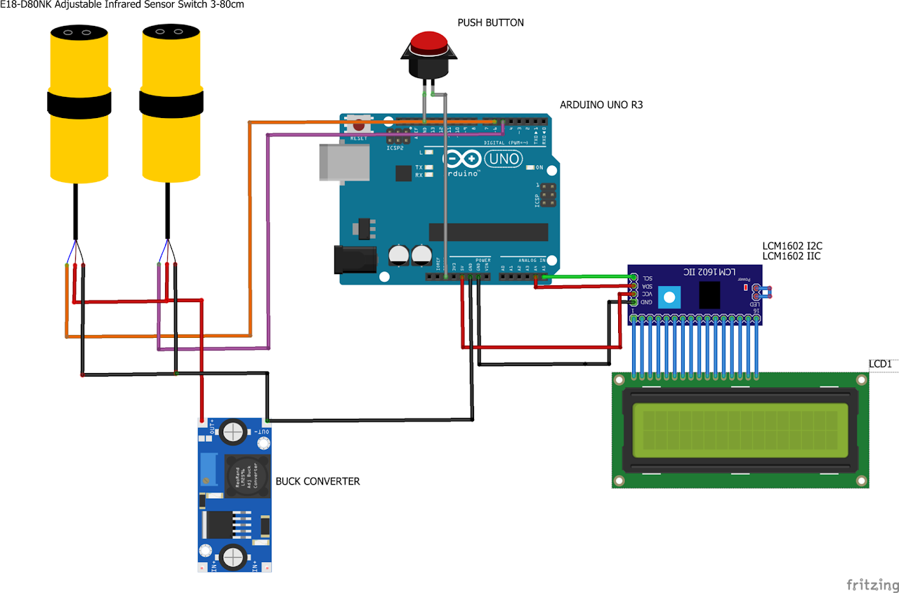
Control code: Control-code-for-Velocity-Measurement-system on GitHub.
06Strain gauges and amplifier
Each bar carries a full Wheatstone bridge at its centre: two gauges along the axis () and two around the circumference (), all on one centreline. Under load the bridge goes out of balance and gives a small voltage:
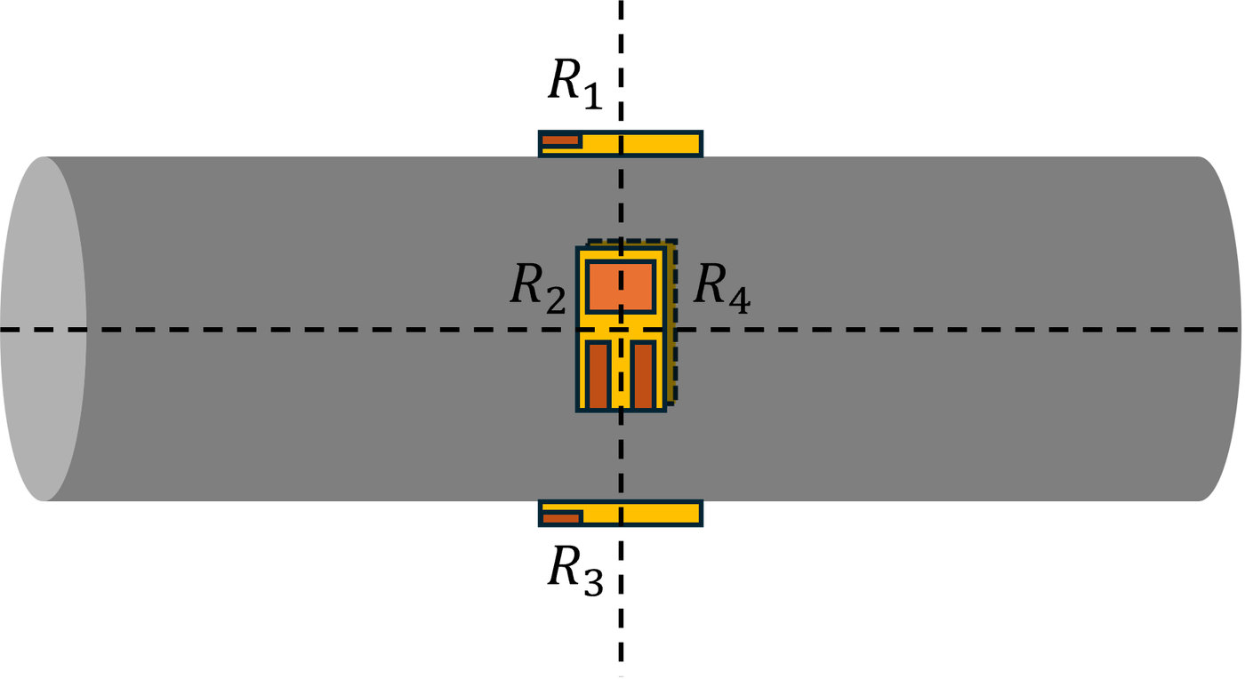
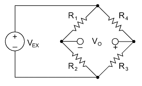
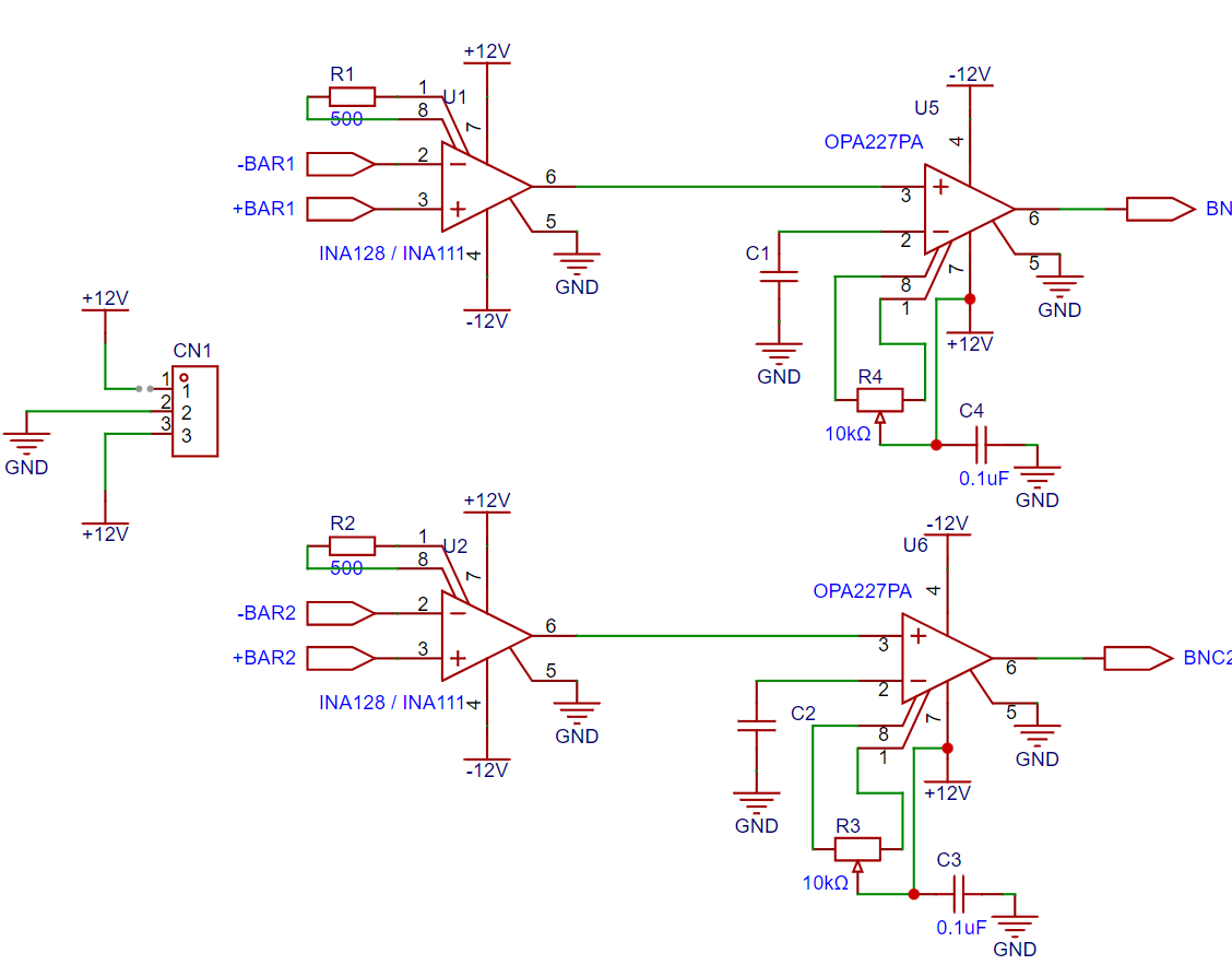
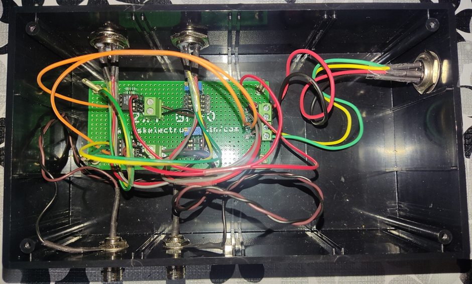
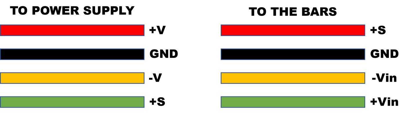
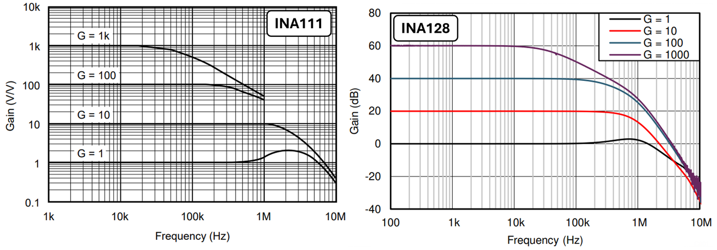
The bridge signal is amplified by a two-channel instrumentation amplifier, one channel per bar. The INA128 (or the faster FET-input INA111) runs at a gain of ×100, set by a 500 Ω resistor between pins 1 and 8; an OPA227 stage and a trimmer remove the DC offset at rest.
From voltage to strain
With excitation , amplifier gain , gauge factor and bridge factor :
For the long–lat–long–lat full bridge the bridge factor is (2.6 for steel). Other layouts: four longitudinal gauges, 4; half bridge or a 0/90° rosette, 2; quarter bridge, 1. With V, , and , strain is .
07Theory
Stress, strain and strain rate in the specimen
With bar wave speed , the particle velocities at the two faces of the specimen are
and the forces on them
When the specimen is in equilibrium (, so ), the classic one-wave relations follow:
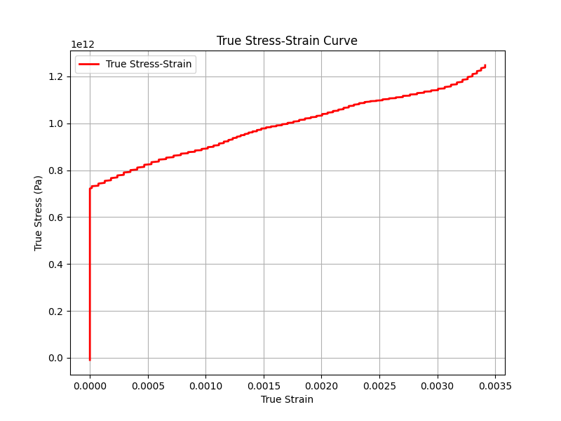
True strain and true stress (compression positive):
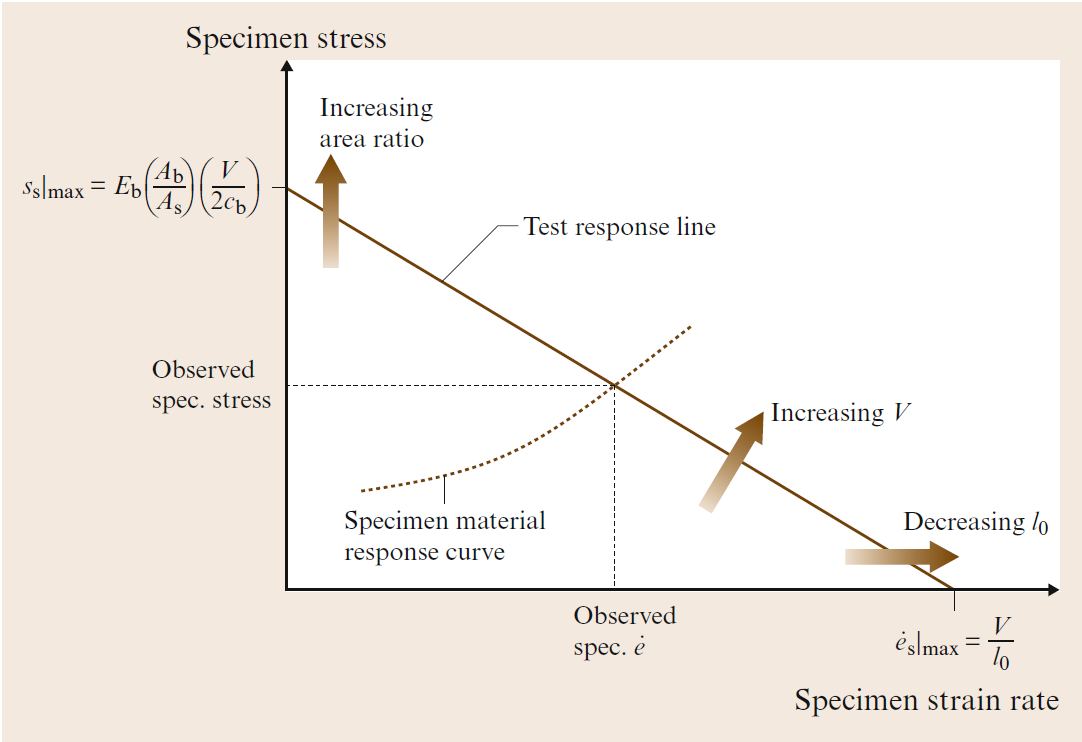
Designing a test: the response diagram
The incident strain is set by the striker velocity, . Combining this with the relations above gives the line every test on a given bar, specimen and velocity must lie on:
The test runs where this line crosses the material's own flow-stress curve. The two ends of the line are the limits: for a material with no strength, and for one that does not flow. So the same set-up drives a strong material at a lower strain rate than a soft one; to reach a chosen point, change the specimen size or the striker velocity.
08Validity checks
- Stress equilibrium: the loading must last much longer than the specimen transit time ; checked by comparing the forces on both faces.
- Friction: friction at the faces stiffens the result, more so at small ; keep between 0.5 and 1 and lubricate with MoS₂ or lithium grease.
- Dispersion: short, sharp pulses spread out along the bars and add oscillations; a pulse shaper between striker and bar lengthens the rise time.
- Inertia: axial and radial inertia add an error to the flow stress that grows with the square of the strain rate:
09Data reduction and results
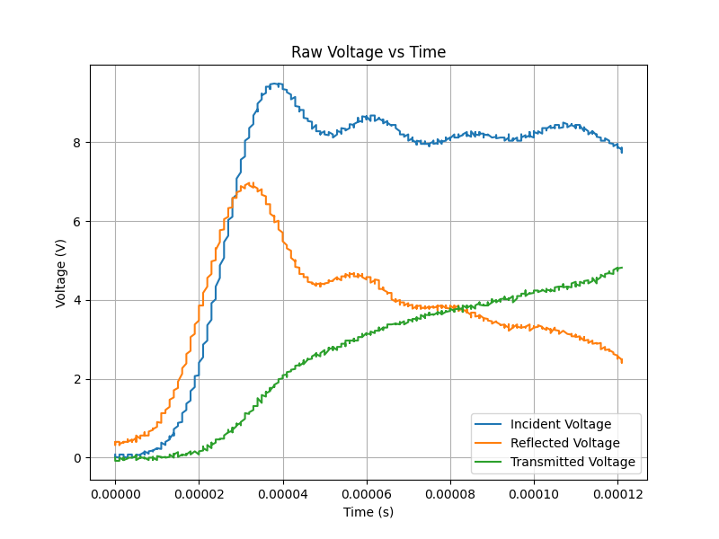
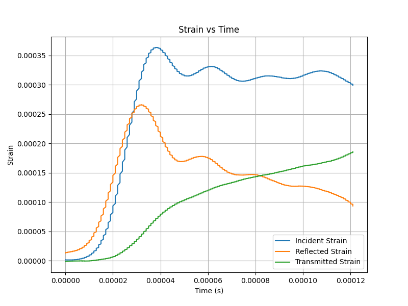
- Crop the recorded voltage–time traces and line up the incident, reflected and transmitted pulses.
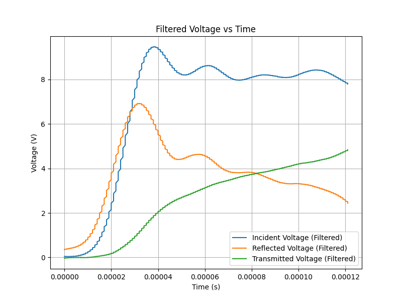
- Smooth them with a Savitzky–Golay filter.
- Convert voltage to strain with the bridge relation.
- Compute particle velocities and the specimen strain rate; integrate it for strain.
- Compute specimen stress from the transmitted pulse, then true stress and true strain.
10Analysis software
The reduction above is packaged twice. The first version is a MATLAB app with a clipping tool for the raw traces and a wave-analysis window (Split-Hopkinson-Pressure-Bar-Analysis-Tool, with a video tutorial). The second is a Python script built on pandas, NumPy, SciPy and Matplotlib (SHPB-Analysis): it reads a CSV or Excel file with time, incident, reflected and transmitted voltages, takes the bar and specimen properties as inputs, and plots the filtered signals, strains, and nominal and true stress–strain curves.
pip install -r requirements.txt
python analysis.py11References
- Ramesh, K. T. (2008). High rates and impact experiments. In Sharpe, W. (ed.), Springer Handbook of Experimental Solid Mechanics. Springer. doi:10.1007/978-0-387-30877-7_33
- Kolsky, H. (1963). Stress Waves in Solids. Dover.
- Chen, W. W., and Song, B. (2011). Split Hopkinson (Kolsky) Bar: Design, Testing and Applications. Springer.
- Lifshitz, J. M., and Leber, H. (1994). Data processing in the split Hopkinson pressure bar tests. International Journal of Impact Engineering, 15(6), 723–733.
- Johnson, W. (1972). Impact Strength of Materials. Edward Arnold.