Split Hopkinson Pressure Bar (SHPB) #
The Split Hopkinson pressure bar (SHPB) is a highly specialized mechanical testing apparatus designed to measure the dynamic behavior and properties of materials under high-strain-rate conditions. Strain rate is the speed at which a material is deformed. SHPBs are used to simulate the kind of forces materials experience during things like car crashes, explosions, and ballistic impacts.
The apparatus, based on devices invented by Bertram Hopkinson and Herbert Kolsky, was developed at SwRI in 1962 by Dr. Ulric Lindholm. Initially created to evaluate the behavior of metals under various conditions, the SwRI Split-Hopkinson Pressure Bar has since been applied to a wide range of materials.
The Kolsky bar, also known as the Split-Hopkinson Pressure Bar (SHPB) experiment, is a well-established technique for assessing the mechanical properties of various materials within the strain rate range of \(10^2 - 10^4 \, \text{s}^{-1}\). A schematic of the experimental setup is depicted in the accompanying figure. This setup comprises two long bars, called the input and output bars, designed to remain elastic throughout the test. These bars enclose a small specimen, typically cylindrical, which is expected to undergo inelastic deformations.
The bars are commonly constructed from high-strength steels such as maraging steel, known for its high yield strength and substantial toughness. One end of the input bar is struck by a projectile made of the same material as the bars. The resulting compressive pulse travels down the input bar toward the specimen. The wave propagation is illustrated in the Lagrangian wave propagation diagram of the figure, where \( t = 0 \) corresponds to the moment of projectile impact.
Within the specimen, multiple reverberations of the loading wave occur. A transmitted pulse is sent into the output bar, while a reflected pulse travels back into the input bar. Typically, resistance strain gauges are affixed to the input and output bars to measure the following:
- The incident pulse generated by the impacting projectile.
- The reflected pulse from the input bar/specimen interface.
- The transmitted pulse through the specimen to the output bar.
It is crucial that the strain gauge locations are chosen so that the incident and reflected pulses do not overlap, as depicted in the accompanying figure.
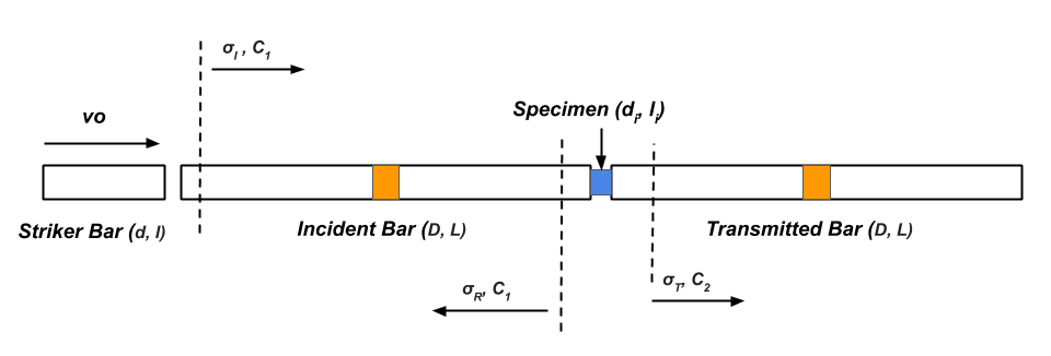
Two-dimensional representation of SHPB
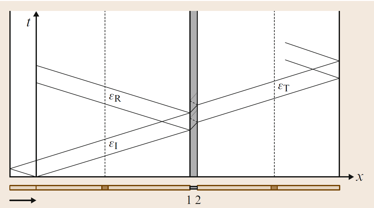
Wave propagation (also called time-distance or Langrangian) diagram showing the stress waves progagating through space and time in SHPB arrangement.
Applications of SHPB #
- Evaluating the behavior of metals, ceramics, composites, polymers, and other materials under various conditions such as impact, explosion, or high-energy events.
- Determining the dynamic strength of materials used in offshore platforms, advanced armors, pipelines, nuclear pressure vessels, space stations, and other high-stress environments.
- Studying material behavior in compression, tension, and shear modes to gain insight into their performance under different loadings.
- Investigating the effects of temperature, strain rate, loading history, and microstructure on material properties for more comprehensive analysis.
- Researching the high-strain-rate behavior of biological tissues to inform medical research and improve protective equipment for human safety.
- Examining advanced materials, such as shape-memory alloys, that require specialized testing under high-strain-rate conditions for engineering applications.
- Testing impact resistance and fracture properties of brittle materials such as ceramics and glass, contributing to the design of safer and more durable products.
- Evaluating materials used in aerospace and automotive industries, providing insights into the structural integrity and crashworthiness of vehicles and aircraft.
- Assessing the impact response of materials used in protective gear and equipment, such as helmets and body armor, to improve safety standards.
Design Rules of SHPB #
- Material Selection: Choose bars and specimens of uniform material properties to ensure accurate wave propagation and measurement.
- Bar Length and Diameter: Optimize the length and diameter of the bars to control the wave propagation characteristics and achieve the desired frequency range and strain rate.
- Alignment and Symmetry: Ensure proper alignment and symmetry of the bars and specimen to minimize measurement errors and enhance test repeatability.
- Specimen Geometry: Select an appropriate specimen geometry (e.g., cylindrical or prismatic) and dimensions that best represent the material behavior under test.
- Strain Gauge Placement: Position strain gauges on the incident and transmitted bars to capture the strain and stress waves accurately.
- Wave Propagation Time: Adjust the bar lengths to control the time it takes for the wave to travel from the impact to the strain gauges, allowing for precise data acquisition.
- Velocity Measurement: Utilize optical or electromagnetic methods to measure the impactor's velocity for accurate analysis of strain rate.
- End Conditions: Apply suitable end conditions (e.g., free or fixed) based on the specific testing requirements to avoid wave reflections and maintain uniform stress distribution.
- Specimen-Machine Interaction: Minimize interaction between the specimen and the SHPB system to prevent errors in data collection and maintain the integrity of the test results.
- Data Acquisition and Analysis: Implement a high-speed data acquisition system to accurately capture the rapid changes in strain and stress during the test, and utilize appropriate software tools for data analysis.
- Safety Measures: Follow safety protocols and guidelines during testing to protect personnel and equipment, especially when working with high-energy or hazardous materials.
Test Conditions of SHPB #
- Temperature Control: Maintain consistent test and specimen temperatures to account for temperature-dependent material properties and avoid thermal gradients that could affect results.
- Humidity Levels: Keep humidity levels low to minimize the impact on the performance of sensors and other electronic components during testing.
- Vibration Minimization: Reduce external vibrations during the test to prevent interference with measurements taken by the strain gauges and other sensors.
- Specimen Alignment: Ensure precise alignment of the specimen with the incident and transmitted bars to guarantee accurate data and consistent stress wave propagation.
- Loading Rate Control: Adjust the loading rate according to the desired strain rate and testing conditions to obtain meaningful data relevant to the material's performance.
- Bar Configuration: Use bar configurations (e.g., bar diameter and length) that suit the specific material and strain rate range to optimize wave propagation and data accuracy.
- Impact Velocity Measurement: Measure the impactor's velocity accurately using optical or other suitable methods to calculate the strain rate and other dynamic parameters.
- Reflection and Dispersion Control: Minimize wave reflections and dispersion in the system by using suitable damping materials and correct bar and specimen geometry.
- Specimen Surface Preparation: Prepare the specimen's surfaces appropriately to ensure even stress distribution and avoid localized stress concentrations or slipping during the test.
- Data Acquisition and Synchronization: Utilize high-speed data acquisition systems and synchronize measurements from different sensors to obtain a complete picture of the specimen's behavior.
- Safety Precautions: Implement safety protocols for personnel and equipment, especially when working with high-energy materials or hazardous conditions during testing.
High Strain-Rate Tests #
One of the defining features of impacts occurring at sufficiently high velocities that cause inelastic, particularly plastic, deformations is that most of these deformations take place at high strain rates. Such deformations may also lead to significant strains and elevated temperatures.
The primary experimental techniques associated with measuring the rate-dependent properties of materials are illustrated in Figure. For the purposes of this discussion, strain rates above \(10^2 \, \text{s}^{-1}\) are classified as high strain rates, while strain rates above \(10^4 \, \text{s}^{-1}\) are termed very high strain rates, and those above \(10^6 \, \text{s}^{-1}\) are known as ultra-high strain rates. Conventionally, strain rates at or below \(10^{-3} \, \text{s}^{-1}\) represent quasistatic deformations, and strain rates below \(10^{-6} \, \text{s}^{-1}\) fall within the creep domain.
Quasistatic experiments are typically carried out using a variety of servohydraulic machines, for which ASTM standards exist to guide most of these tests. Most servohydraulic machines are incapable of consistently achieving strain rates larger than \(100 \, \text{s}^{-1}\); however, some specialized servohydraulic machines can reach strain rates of \(10^1 \, \text{s}^{-1}\). The intermediate strain rate domain, between \(100 \, \text{s}^{-1}\) and \(10^2 \, \text{s}^{-1}\), is particularly challenging to study due to the relevance of wave propagation effects, which are difficult to account for. Nevertheless, this strain rate range holds interest for a variety of machining problems. Drop towers or drop weight machines are the primary means of testing in this range, though careful interpretation of the data is necessary due to the coupling of impact-induced wave propagation with machine vibrations.
In the experimental section, we focus on techniques for studying high strain rates (greater than \(10^2 \, \text{s}^{-1}\)), including the high (\(10^2 - 10^4 \, \text{s}^{-1}\)).
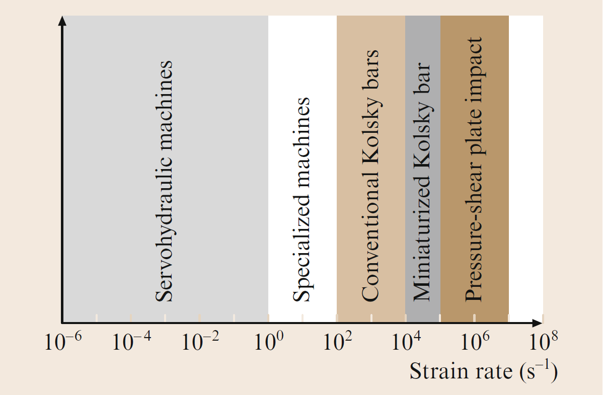
Experimental techniques used for the development of controlled high strain rate deformations in materials
Design of SHPB #
The Split Hopkinson Pressure Bar (SHPB) setup is meticulously designed to ensure precision, stability, and safety during high-velocity impact experiments. Comprising several crucial components, each part plays a pivotal role in the seamless operation of the system.
The SHPB setup is anchored on a robust I-beam structure, providing a sturdy foundation for the entire apparatus. This I-beam serves as the backbone onto which all key elements are securely mounted.
Positioned on the I-beam are dedicated holders for the gas gun and the incident and transmitted bars. These holders are intricately engineered to align the centerline of the gas gun barrel precisely with that of the bars, ensuring optimal performance and accurate data acquisition.
Elevating the I-beam to an optimal height is a 4-meter ladder frame, meticulously crafted to provide essential structural support. This ladder frame offers stability and rigidity to the SHPB setup, crucial for maintaining experimental integrity.
To further enhance stability and ensure the rigidity of the entire system, a series of five A-frames are strategically positioned around the setup. These A-frames, meticulously crafted for maximum strength, provide additional support and sturdiness to the SHPB apparatus.
Ensuring precise alignment and balance of the SHPB setup is the incorporation of leveling screws at the base of each A-frame leg. These screws allow for fine adjustments, enabling operators to calibrate the system with meticulous accuracy.
CAD parts of SHPB setup
CAD assembly of SHPB setup
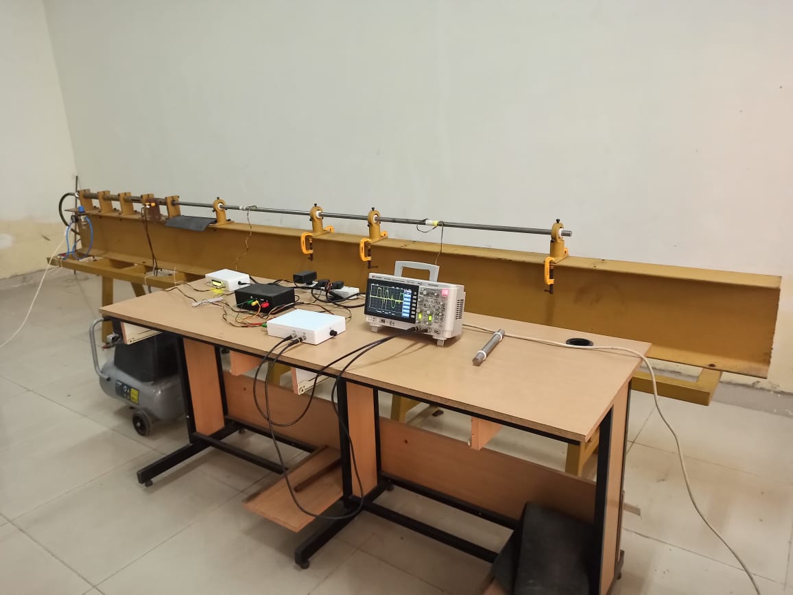
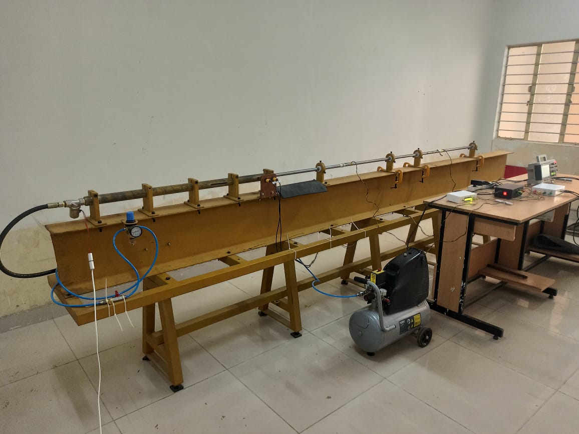
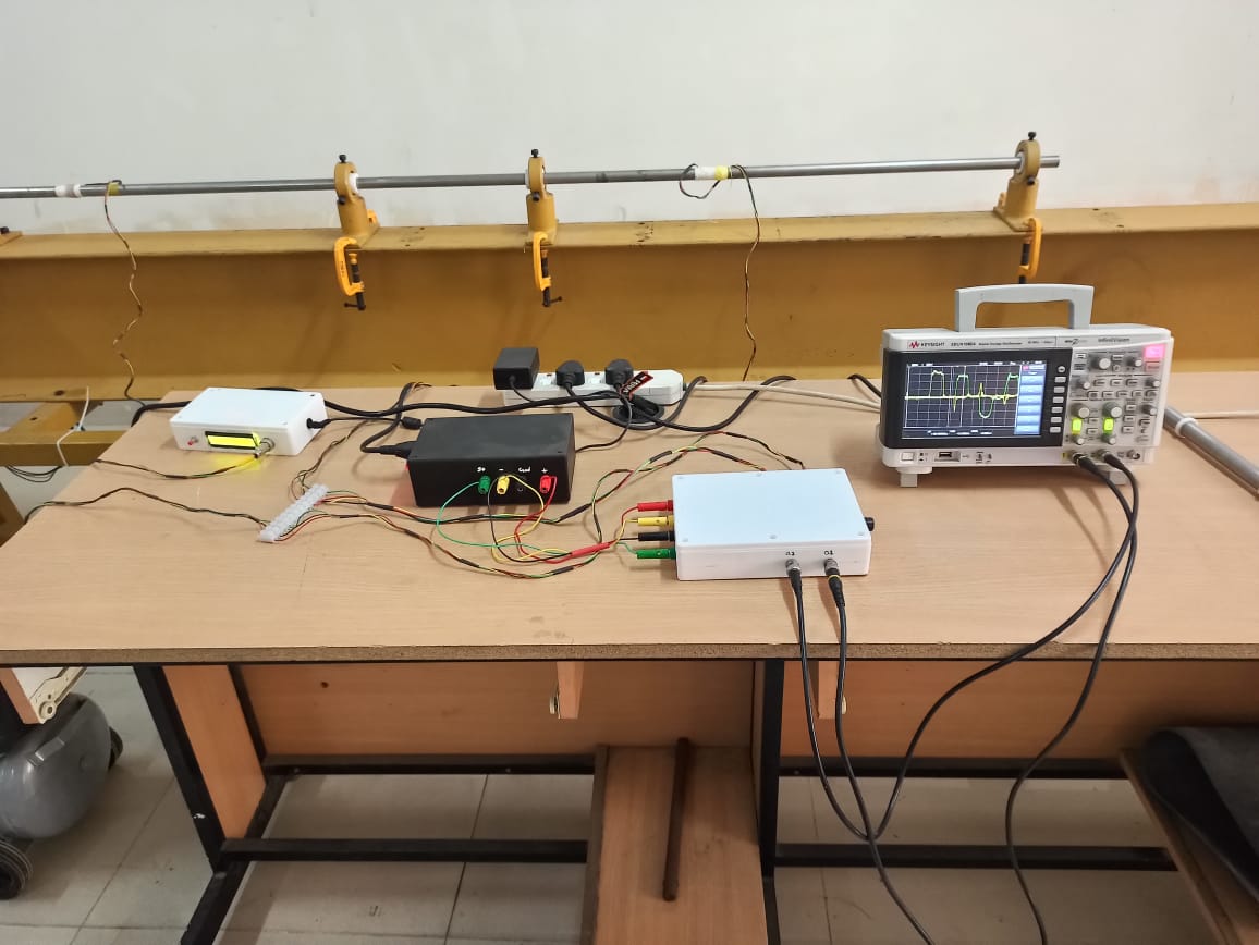
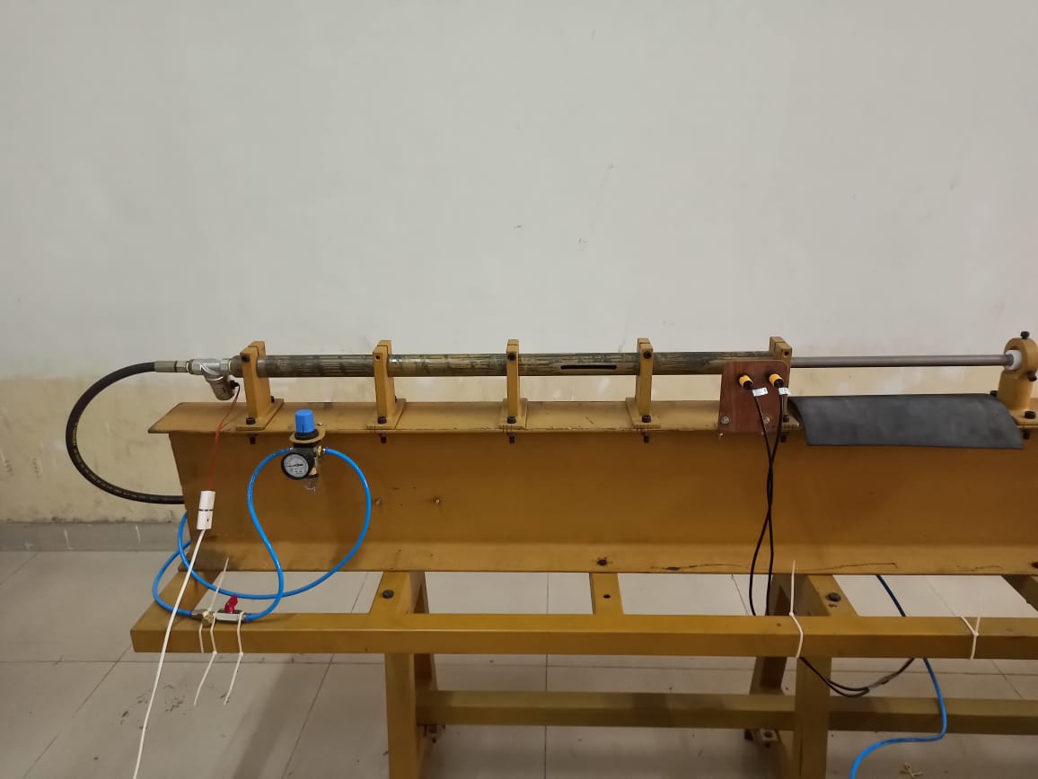
Experimental Setup #
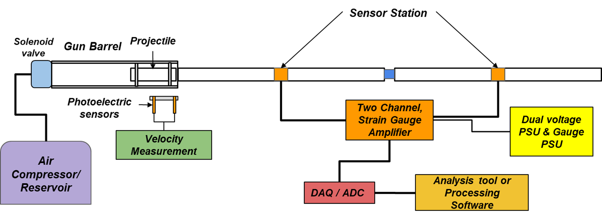
Outline of SHPB
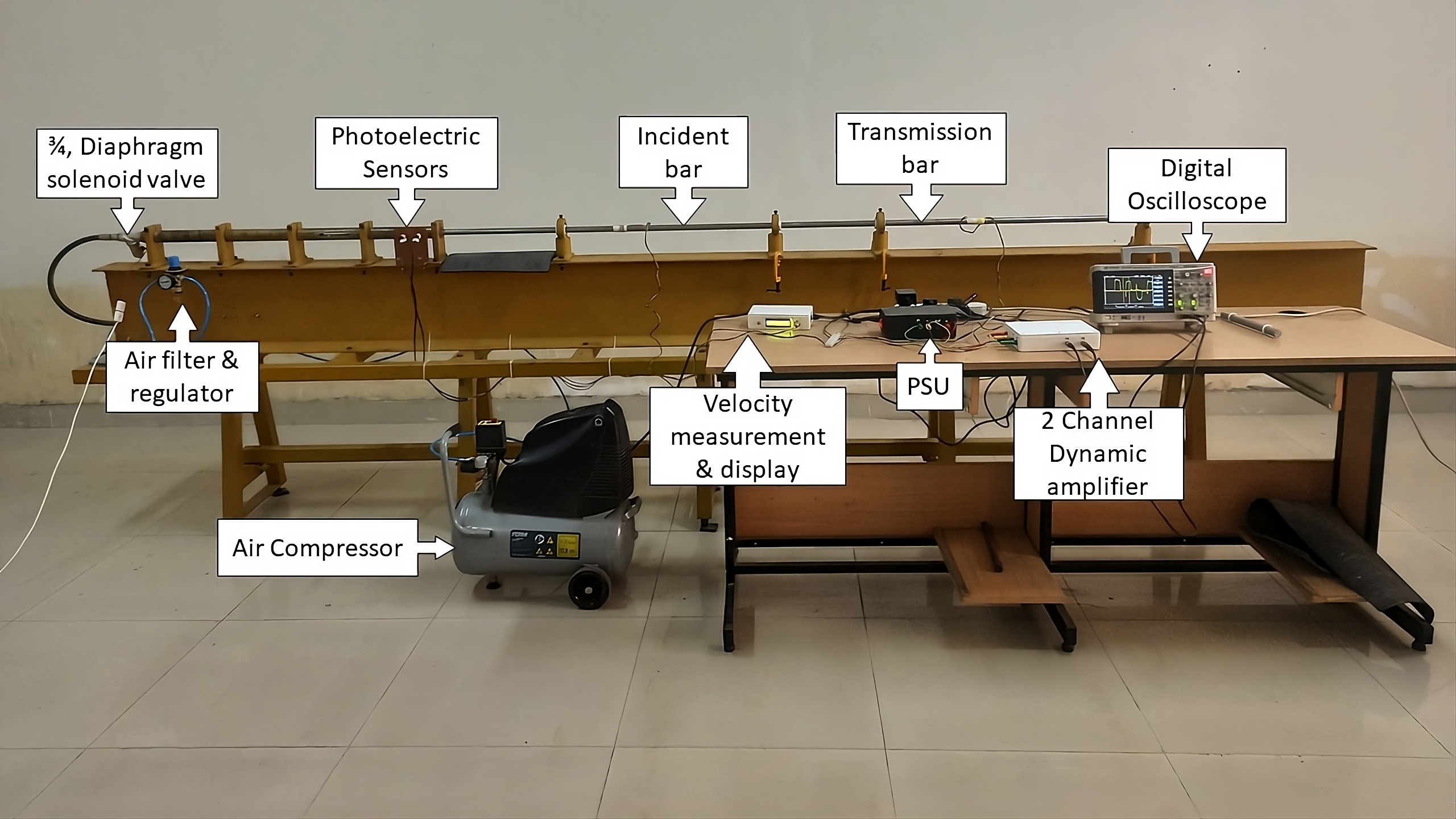
Annotated Setup of SHPB
Setup Images of SHPB
Striker Launch System #
The gas gun, also known as the striker launch system, is a critical component in high strain-rate experiments, such as those performed with the Split Hopkinson Pressure Bar (SHPB) setup. This system is used to propel the striker bar toward the Incident bar at set speeds which picks up the stress pulse that direct towards the specimen. The gas gun is designed to launch the striker bar at controlled speeds, simulating the high strain-rate conditions materials may experience in real-world scenarios. By adjusting the pressure within the gas gun, the launch speed can be fine-tuned and the energy imparted to the striker bar, enabling precise control over the impact force and strain rates experienced by the test specimen.
The gas gun uses pressurized gas to accelerate the striker bar. The striker bar is launched towards the test incident bar, creating an impact that generates stress waves in the bars that travel to the specimen and the trasmitted bar. This system operates through the careful control and release of compressed air to propel the striker bar down a barrel. Here’s how the system is designed and functions:
- Air Compression: The process begins with an air compressor, which fills up air in a containment cylinder. This allows for the storage and management of compressed air for use in the system.
- Airflow Control and Filter: The outlet of the air compressor's cylinder is connected to an air flow controller and filter, which are in conjunction with a ball valve. This setup ensures that air can only be released when the cylinder is filled with compressed air.
- Reservoir Tank: The air flow controller and filter are equipped with a non-return NC (normally closed) valve, ensuring one-way airflow. This is then connected to a reservoir tank, which can be filled with the exact pressure of compressed air needed for launching the striker bar at a specific speed.
- Hydraulic Hose Connection: The reservoir is linked to the gas gun barrel via a 3/8 inch, 180-bar hydraulic hose. This ensures a secure connection and the efficient transfer of compressed air from the reservoir to the barrel.
- Solenoid Valve Activation: At the junction between the barrel and the hose is a 3/4 inch semi-lift diaphragm solenoid valve (NC). This valve is controlled by a 220V AC power supply and is triggered by a button.
- Striker Bar Propulsion: When the button is pressed, the solenoid valve opens, allowing compressed air from the reservoir to enter the barrel. This sudden influx of air propels the striker bar at high speed down the barrel.
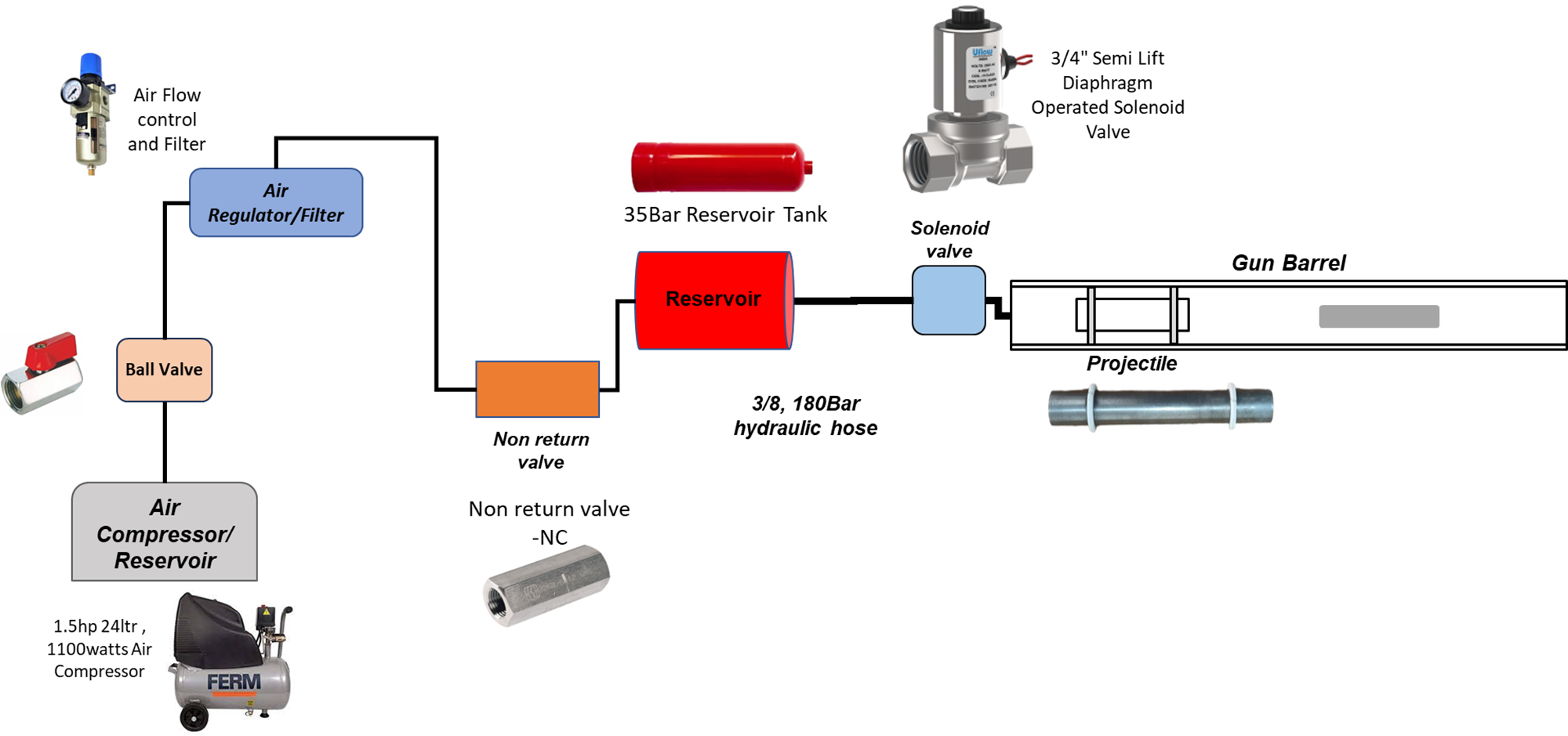
Fig: Outline of Striker Launch System
Calculation of Striker Velocity Based on Air Pressure Set at Release from Reservoir #
This precise and controlled operation of the striker launch system is crucial for performing reliable and accurate experimental tests involving high strain rates. To calculate the velocity of the striker based on the air pressure set at release from the reservoir, follow these steps:
- Note the mass \( m_s \) and length \( l_s \) of the striker/impactor.
- Note the displacement \( s_s \) of the striker in the barrel.
- Calculate the area of the barrel \( A_b \) using the known diameter of the gas gun barrel \( d_b \).
- Note the pressure of the compressed air \( P \) in the reservoir.
- Calculate the force exerted on the striker based on the noted pressure and area of the barrel:
\[ P = \frac{F}{A} \]
Rearranging terms, \[ F = P \cdot A_b \] (\(Pascal \cdot m^2 \)) \( \left(\frac{kg}{ms^2}\right) \cdot m^2 = \frac{kg \cdot m}{s^2} \) - Force is also expressed as a product of mass times acceleration, \( F=ma. \)
- Rearranging the terms to calculate the acceleration of the striker using the formula:
\[ a = \frac{F}{m_s} \]
\( \left(\frac{kg \cdot m}{s^2}\right) \cdot \left(\frac{1}{kg}\right) = \frac{m}{s^2} \) - Calculate the striker's velocity from the equation of motion:
\[ v_s = \sqrt{2 \cdot a \cdot s_s} \]
\( \sqrt{\left(\frac{m^2}{s^2}\right)} = \frac{m}{s} \)
Striker Velocity Calculator
Velocity Measurement System for Stiker Bar #
The Velocity Measurement System utilizes two closely positioned infrared sensors to accurately measure the time delay between sensor triggers. The system features a 16x2 LCD that displays the time interval in microseconds (µs) and the calculated velocity in meters per second (m/s).
As an object passes through the infrared sensors, the system records the time difference between the triggers of the two sensors. By noting the known distance between the sensors and the recorded time difference, the system calculates the object's velocity. The microcontroller captures the precise times at which the sensors are triggered, allowing for precise measurement of the time taken for the object to traverse the distance between the sensors. The system then computes the velocity by dividing the distance by the time interval.
The velocity measurement system is governed by an Arduino Uno microcontroller, which orchestrates the system's operations. Initially, the infrared sensors detect the signal trigger generated by the moving object, transmitting this information to the Arduino Uno. The distance between the sensors is pre-established and remains fixed throughout the measurement process.
Upon the detection of the signal trigger, the system records the time delay, denoted as \( t \), between the activation of the two sensors, \( t_1 \) and \( t_2 \). This time delay is crucial for determining the speed of the projectile traversing between the two sensors. The predefined distance \( d \) separating the sensors is set at 50mm.
The velocity \( v \), of the projectile is then calculated using the fundamental equation: \[ v = \frac{d}{t} \] Here, \( v \) represents the velocity, \( d \) signifies the distance between the sensors, and \( t\) corresponds to the time taken for the projectile to pass from the first to the second sensor.
The velocity measurement system is powered by a specialized Arduino code designed to optimize its functionality. The circuit simulator diagram below illustrates the components and connections integral to the system's operation. Following the diagram, you will find the control code used to calculate and display the speed in meters per second (m/s).
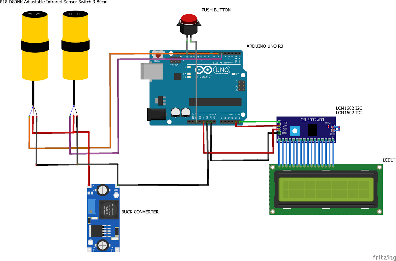
Fig: Circuit Simulator outline of Velocity Measurement System
            #include < Wire.h >                                // I2C Communication library
            #include < LiquidCrystal_I2C.h >                   // LCD with I2C library

            LiquidCrystal_I2C lcd(0x27, 16, 2);

            int S1 = A2; // Analog Pin 2
            int S2 = A3; // Analog Pin 3

            int val1; // Value Store for S1
            int val2; // Value Store for S2

            int threshold;
            unsigned long time1, time2;
            float Time, Speed;

            byte customChar[] = {
                B00000,
                B00100,
                B01010,
                B10001,
                B10001,
                B10001,
                B11111,
                B00000
            };

            void setup() {
                Serial.begin(9600);
                pinMode(S1, INPUT);
                pinMode(S2, INPUT);

                val1 = digitalRead(S1);
                val2 = digitalRead(S2);

                threshold = (((val1 + val2) / 2) + 45);

                lcd.init();
                lcd.backlight();
                lcd.setCursor(0, 0);
                lcd.clear();

                lcd.createChar(0, customChar);
                lcd.home();
                lcd.write(0);
                lcd.setCursor(1, 0);
                lcd.print("t=");

                lcd.setCursor(0, 1);
                lcd.print("V =");
            }

            void loop() {
                val1 = analogRead(S1);
                val2 = analogRead(S2);

                while (val1 <= threshold) {
                    val1 = analogRead(S1);
                }

                while (val1 > threshold) {
                    time1 = micros();
                    val1 = analogRead(S1);
                }

                while (val2 <= threshold) {
                    val2 = analogRead(S2);
                }

                while (val2 > threshold) {
                    time2 = micros();
                    val2 = analogRead(S2);
                }

                Time = time2 - time1;
                Speed = (50000 / Time); // 50mm - Distance between two sensors

                Serial.print(Time);
                Serial.println(Speed);

                lcd.setCursor(3, 0);
                lcd.print(Time);
                lcd.setCursor(12, 0);
                lcd.print("us");
                lcd.setCursor(3, 1);
                lcd.print(Speed);
                lcd.setCursor(8, 1);
                lcd.print("m/s");
            }
Signal Amplification #
Signal / Voltage amplification is a system that often utilizes amplifiers, an instrumentation device designed to detect and amplify minute voltage changes. This device measures variations in electrical resistance caused by an external force or pressure, enabling the quantification of parameters such as force, pressure, tension, and weight.
The INA111 is a high-speed, FET-input instrumentation amplifier that provides superior performance, making it a valuable component for advanced applications. For low-power, general-purpose applications, the INA128 offers exceptional accuracy and is a reliable choice. A gain setting of x100 is recommended, achieved by connecting a 500Ω resistor between pin 1 and pin 8 of the operational amplifier. The OPA227 series operational amplifiers combine low noise and wide bandwidth with high precision to make them the ideal choice for applications requiring both AC and precision DC performance. The trimmer potentiometer can be adjusted to nullify the DC offset in the output signal under static conditions.
The SHPB experiment utilises data from two distinct bars: the incident and transmitted bars. To achieve accurate readings, two separate strain gauge amplification circuits are constructed. These circuits will enhance the signals from each bar, providing a precise representation of the data collected. This setup ensures a robust measurement system capable of delivering consistent and reliable results.
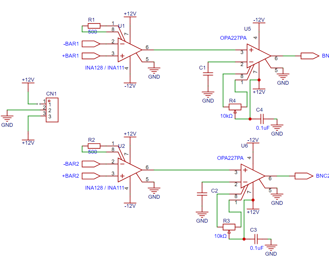
2-Channel Strain Gauge Amplifier-Circuit
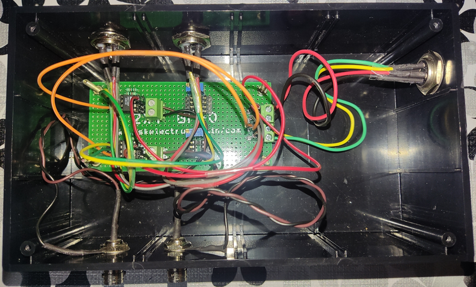
2-Channel Amplifier Circuitry-Image

Amplifier Wiring Colour Schematic
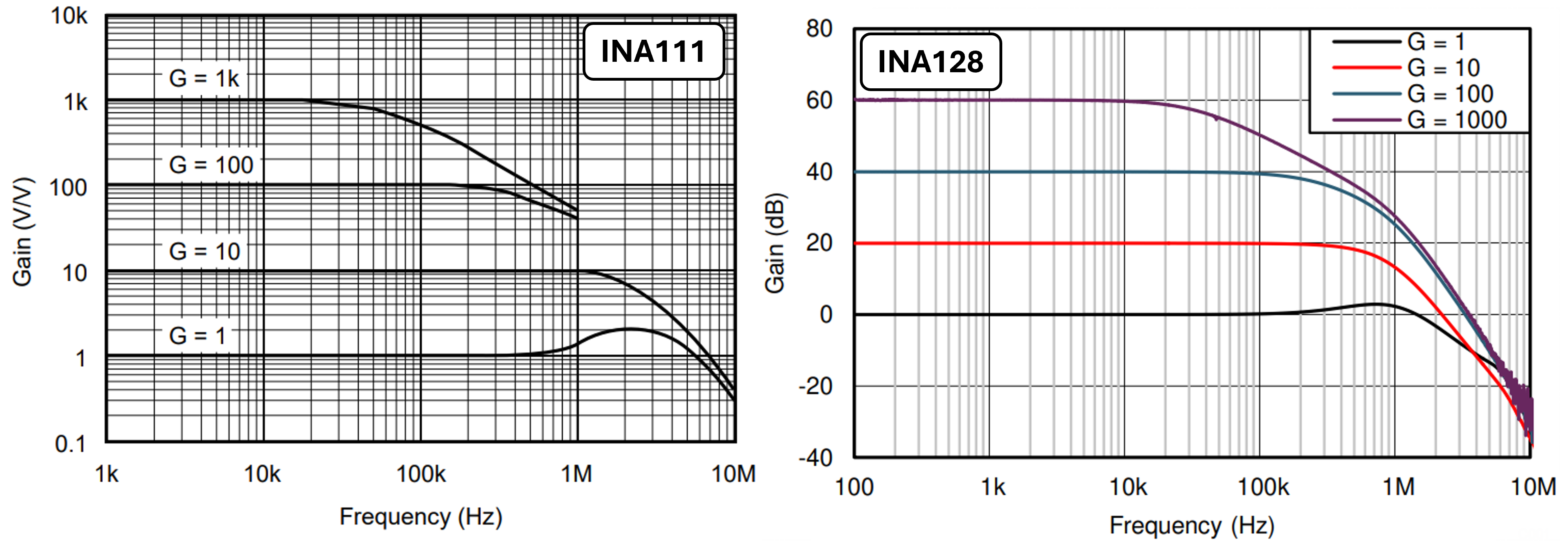
Gain -Frequency Comparison for INA111 and INA128
Links to Datasheets
Theory of SHPB #
Design Theory of SHPB Experiment
The design of a specific Kolsky bar experiment is fundamentally centered around two key aspects: the specimen design and the projectile impact velocity selection. These factors are pivotal in achieving the desired strain rate within the specimen, thereby facilitating accurate data acquisition and analysis.
Among the design parameters, the choice of specimen length (\( l_0 \)) and diameter (\( d_0 \)) holds paramount importance. Additionally, the selection of the projectile impact velocity plays a crucial role in achieving the desired strain rate. Other design parameters such as the bar length (\( L \)) and bar diameter (\( D \)) are more relevant to the overall design of the Kolsky bar system rather than the specific experiment.
Three critical ratios dictate the design considerations: \( \frac{L}{D} \), \( \frac{D}{d_0} \), and \( \frac{l_0}{d_0} \). Typically, the ratio \( \frac{L}{D} \) falls within the range of approximately 100, while \( \frac{D}{d_0} \) typically ranges from 2 to 4. The ratio \( \frac{l_0}{d_0} \) typically ranges from 0.6 to 1.
The selection of the bar diameter (\( D \)) is contingent upon several factors, including the material under test, the availability of typical specimen sizes, and the permissible degree of wave dispersion. While a larger value of \( \frac{D}{d_0} \) allows for the testing of harder specimen materials, it's essential to consider the interface between the specimen and the bar. The expectation that this interface can be approximated as a plane imposes limitations on the value of \( \frac{D}{d_0} \).
Experimental Design Approach
A systematic approach to experimental design is outlined below. The strain in the incident pulse (\( \varepsilon_1 \)) is given by:
\[ \varepsilon_1 = \frac{V}{2C_b} \]
Where \( V \) represents the projectile velocity. Utilizing this equation along with the equilibrium condition (\( P_1 = P_2 \)) and \( S_s(t) = \frac{E_b A_b}{A_s} \varepsilon_T(t) \), we can express the specimen stress entirely in terms of the reflected strain and the impact velocity:
\[ S_s(t) = \frac{E_b A_b}{A_s} \varepsilon_T(t) = \left( \frac{E_b A_b}{A_s} \right) (\varepsilon_I + \varepsilon_R) = \left( \frac{E_b A_b}{A_s} \right) \left( \frac{V}{2C_b} + \varepsilon_R \right) \]However, the equation \[ \dot{e}_s(t) = \frac{2c_b}{l_0} \varepsilon_R(t) \] allows us to express the strain in the reflected pulse in terms of the specimen strain rate:
\[ \varepsilon_R = -\frac{l_0}{2C_b} \dot{e}_s \]
Using this in the previous equation, we obtain the relation between the specimen stress and the specimen strain rate that must be satisfied during any given test using a specific Kolsky bar, a specific specimen, and a particular choice of impact velocity:
\[ S_s(t) = Eb \cdot \left( \frac{{A_b}}{{A_s}} \right) \cdot \left( \frac{{V}}{{2C_b}} \right) - Eb \cdot \left( \frac{{A_b}}{{A_s}} \right) \cdot \left( \frac{{lo}}{{2C_b}} \right) \cdot \dot{e}_s \]This last result represents what we call a test characteristic response: that is, the constraints of the experimental configuration force any observed stresses and strain rates in the specimen to satisfy. The result is shown as the straight line in the figure, which is a plot of the stress versus the strain-rate (hereafter called a response diagram). Note that in this figure compressive stresses are presented along the positive Y-axis, following our convention. The straight line represents the locus of all points in stress versus strain-rate space that can be reached using a compression Kolsky bar, a specific specimen geometry, and a specific projectile impact velocity. The figure also shows the curve corresponding to the constitutive response of the specimen material (typically, the flow stress increases with strain-rate). The stresses and strain rates actually observed in a given test correspond to the intersection of the test response line with the constitutive curve. In the context of material testing, the constitutive response reflects the inherent behavior of the material under varying conditions, such as strain rate.
Unlike experimental parameters that can be controlled, such as specimen geometry and impact velocity, the constitutive response of the material remains fixed. Achieving specific strain rates during testing requires adjusting the test response line, representing the experimental parameters. To explore different points along the constitutive curve, corresponding to varying material behaviors, the straight line indicative of the experimental setup needs to be shifted accordingly.
The above Equation indicates that the maximum strain rate that can be observed in a SHPB test is given by:
\[\dot{e}_s|_\text{max} = \frac{V}{l_0}\]
while the maximum compressive stress that can be observed in such a test is given by
\[S_s|_\text{max} = E_b \left(\frac{A_b}{A_s}\right) \left(\frac{V}{2C_b}\right)\]
The figure illustrates that reaching the maximum strain rate is only feasible in an actual Kolsky bar test if the material exhibits an extremely soft response, resulting in the observed specimen stress approaching zero. Conversely, attaining the maximum specimen stress in the test is only possible when the specimen strain rate is nearly zero. This phenomenon mathematically reflects the well-established principle that a specific test procedure tends to yield lower strain rates for strong materials, while very soft materials can deform at significantly higher strain rates under identical testing conditions.
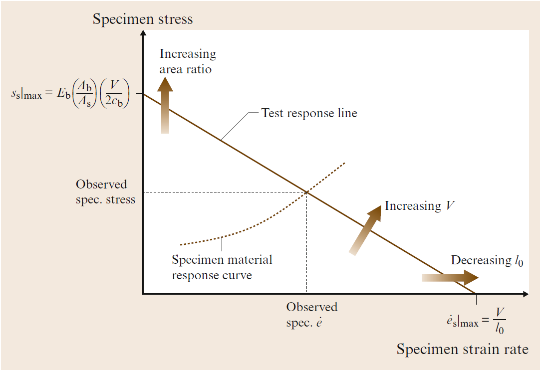
Response diagram for the compression Kolsky bar, showing the intersection of the material response curve (dashed) with the test response line
Explanation for Stress-Strain Calculation in SHPB Experiment
In the Split Hopkinson Pressure Bar (SHPB) experiment, the characteristic relations associated with one-dimensional elastic wave propagation in the bar provide the basis for calculating stress and strain in the specimen.
1. Particle Velocity at Specimen/Input-Bar and Specimen/Output-Bar Interface
- The particle velocity \( v_1(t) \) at the specimen/input-bar interface is given by:
\[ v_1(t) = c_b (\varepsilon_I - \varepsilon_R) \]
Here, \( c_b = \sqrt{\frac{E_b}{\rho_b}} \) represents the bar wave speed, with \( E_b \) denoting the Young's modulus and \( \rho_b \) the density of the bar material.
- The particle velocity \( v_2(t) \) at the specimen/output-bar interface is given by:
\[ v_2(t) = c_b \varepsilon_T \]
2. Mean Axial Strain Rate in the Specimen
- The mean axial strain rate \( \dot{e}_s \) in the specimen is calculated as:
\[ \dot{e}_s = \frac{c_b}{l_0} (\varepsilon_I - \varepsilon_R - \varepsilon_T) = \frac{v_1 - v_2}{l_0} \]
Here, \( l_0 \) represents the initial specimen length.
3. Calculation of Bar Stresses and Normal Forces
- The stresses and normal forces at the specimen/bar interfaces are computed as follows:
\[ P_1 = E_b (\varepsilon_I + \varepsilon_R) A_b \] at the specimen/input-bar interface.
\[ P_2 = E_b \varepsilon_T A_b \] at the specimen/output-bar interface.
Here, \( A_b \) denotes the cross-sectional area of the bars.
4. Mean Axial Stress in the Specimen
- The mean axial stress \( \bar{S}_s(t) \) in the specimen is given by:
\[ \bar{S}_s(t) = \frac{(P_1 + P_2)}{2} \left( \frac{1}{A_s} \right) \]
Here, \( A_s \) represents the initial cross-sectional area of the specimen.
5. Stress-Strain Relationship
- Assuming stress equilibrium, uniaxial stress conditions in the specimen, and one-dimensional elastic stress wave propagation without dispersion in the bars, the nominal strain rate \( \dot{e}_s \), nominal strain \( e_s \), and nominal stress \( S_s \) in the specimen are estimated using:
\[ \dot{e}_s(t) = \frac{2c_b}{l_0} \varepsilon_R(t) \]
\[ e_s(t) = \int_0^t \dot{e}_s(\tau) d\tau \]
\[ S_s(t) = \frac{E_b A_b}{A_s} \varepsilon_T(t) \]
6. True Stress-Strain
- True strain \( \varepsilon_s(t) \) in the specimen is given by:
\[ \varepsilon_s(t) = -\ln(1 - e_s(t)) \]
Here, \( e_s(t) \) represents the engineering strain in the specimen.
- The true strain rate \( \dot{\varepsilon}_s(t) \) in the specimen is calculated as:
\[ \dot{\varepsilon}_s(t) = \frac{\dot{e}_s(t)}{1 - e_s(t)} \]
- The true stress \( \sigma_s(t) \) in the specimen is obtained as:
\[ \sigma_s(t) = S_s(t) \cdot (1 - e_s(t)) \]
Here, \( S_s(t) \) represents the nominal stress in the specimen.
- The resulting True Stress \( \sigma_s(t) \) - True Strain can be plotted
Validation of SHPB Experiments
Several fundamental prerequisites must be met to ensure that the observed response in a SHPB experiment accurately represents the constitutive behavior of the specimen material. The outline each of these requirements is discussed briefly.
Equilibrated Stresses
In SHPB bar experiments, loading initially impacts one side of the specimen. Due to the finite propagation speed of stress waves within the specimen, it takes some time for stresses to equilibrate. This equilibration is essential to ensure that the stress measured at the output side of the specimen accurately represents its average stress state. From an experimental standpoint, stress equilibration occurs when the loading duration is significantly longer than the specimen's characteristic time \(\tau_s = \frac{c_{sp}}{l_0}\), which denotes the time taken for a compressive wave to traverse the specimen's length.
Ensuring equilibrium of axial stress at the desired time is crucial for the effective application of any Kolsky bar method. Typically, equilibrium verification involves comparing the force histories on both sides of the specimen.
Friction Effects
Friction at the interfaces between the specimen and the bars can disrupt the intended uniaxial stress condition, leading to artificially stiff results. This effect becomes more pronounced as the ratio of specimen length to diameter \( l_0/d_o \) decreases. In conventional compression Kolsky bar tests, \( l_0/d_o \) ratios typically range from 0.5 to 1.0, as recommended by Bertholf and Karnes.
The degree of interfacial friction is influenced by various factors, including the smoothness of the end surfaces, the materials of the bars and specimen, the type of lubricant used, impact velocity, and temperature. Commonly employed lubricants in Kolsky bar experiments include \( Mo S_2 \) lubricants and lithium greases.
Dispersion Effects
Longitudinal waves traveling through elastic bars are subject to geometric dispersion, causing changes in the incident, reflected, and transmitted pulses as they propagate along the input and output bars. The phenomenon of wave dispersion has a significant impact on the measured strain pulses, consequently affecting the observed stress-strain response. While dispersion effects can be accurately accounted for through elastic wave propagation computations, two key consequences of dispersion are noteworthy.
Firstly, dispersion inherently introduces superimposed oscillations in the loading of the specimen. Secondly, shorter stress pulses characterized by sharper rise times exhibit greater dispersion due to their higher frequency content and wider range of frequencies.
To mitigate the influence of dispersion, one strategy involves the utilization of buffer materials or shaper materials positioned between the impacting projectile and the input bar. This approach facilitates the modification of the incident wave by extending its rise time, thereby reducing dispersion effects.
Inertial Effects
The stresses induced by axial and radial inertia must be kept minimal in comparison to the flow stress of the material being studied. In high-strain-rate experiments employing stress wave loading, the impact of inertia on measured properties becomes notable, especially at extremely high strain rates.
The extent of the inertial effect on the apparent stress is also contingent upon the density and dimensions of the specimen. The inertial effect in SHPB experiments that can be rewritten to emphasize specimen size and l/d ratio effects as follows:
\[ r = \frac{\sigma_{s_2} - \sigma_y}{\sigma_y} = \frac{\rho d^2}{\sigma_y} \left[ \frac{1}{64} + \frac{1}{6} \left( \frac{l_0}{d_0} \right)^2 \right] \dot{\varepsilon}^2 \]
\( r \) is the relative error in flow stress measurement due to inertia.
\( \sigma_{s_2} \) and \( \sigma_y \) are the flow stress measured from the output bar and the actual yield stress of the material respectively.
\( \rho \) is the density of the specimen material
A practical method to address inertial effects is to determine the maximum achievable strain rate while maintaining the inertial relative error \(r\) within a specified tolerance. This can be achieved by establishing a relationship between the limiting strain rate, the specimen length, and the specific strength \( \frac{\sigma_y}{\rho} \) for the given ratio of \( l_o/d_o \) as:
\[ \dot{\varepsilon}_{lim} = \frac{l}{l_0} \sqrt{\frac{\sigma_y}{\rho} r \left( \frac{192}{32 + \left( \frac{3}{\beta^2} \right)} \right)} \]
where, \( \beta = l_o/d_o \).
Measuring Strain with Strain Gauges
In mechanical testing and measurement, it's crucial to comprehend how materials respond to applied forces. Strain refers to the amount of deformation experienced by a material when subjected to such forces. It's essentially the ratio of the change in length of a material to its original, unaffected length.
Strain can be either positive (tensile) or negative (compressive). Positive strain occurs when a material elongates due to applied force, while negative strain occurs when it contracts.
When a material is compressed in one direction, it tends to expand in directions perpendicular to the applied force. This phenomenon is known as the Poisson effect. Poisson's ratio (denoted as \( \nu \))quantifies this effect and is defined as the negative ratio of transverse strain to axial strain.
Strain is typically expressed as a dimensionless quantity. However, it's sometimes denoted in units such as inches per inch (in./in.) or millimeters per millimeter (mm/mm). Due to the small magnitude of measured strain, it's often represented in microstrain \( \mu\varepsilon \), where one microstrain is equal to \( 10^{-6} \) strain.
Strain gauge, often written as "strain gage," is a common tool used to measure strain in materials. It operates by monitoring changes in electrical resistance when subjected to axial, bending, shear, or torsional forces. As the applied force causes deformation in the material, the electrical resistance of the strain gauge changes proportionally, allowing for the quantification of strain.
The most prevalent type of strain gauge is the bonded metallic strain gauge. This gauge typically comprises a fine wire or metallic foil arranged in a grid pattern. The grid design ensures maximum sensitivity to strain in the parallel direction. This grid is affixed to a thin backing called the carrier, which is directly bonded to the test specimen.
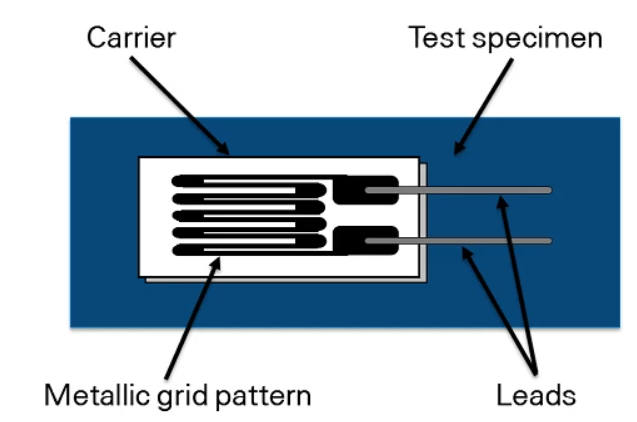
The electrical resistance of metallic grid changes in proportion to the amount of strain experienced by the test specimen.
When the test specimen undergoes strain, this deformation is transmitted directly to the strain gauge via the carrier. Consequently, the strain gauge exhibits a linear alteration in its electrical resistance in response to the strain experienced by the material.
Wheatstone Bridge Theory in Strain Gauge Measurements
The Wheatstone bridge is a fundamental circuit extensively utilized in strain gauge measurements, enabling precise determination of mechanical strain or deformation. Strain gauges, sensitive elements that change resistance in response to mechanical strain, are often employed in bridge configurations due to their high sensitivity and ability to detect subtle changes.
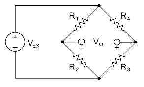
Strain gauges are configured in Wheatstone bridge circuit
In the Wheatstone bridge setup with strain gauges, balance occurs when the ratio of resistances in one voltage divider circuit matches the ratio in the other voltage divider circuit. Specifically, the bridge is balanced when:
\[ \frac{R_1}{R_2} = \frac{R_4}{R_3} \]
Achieving this balance ensures that any external disturbances, such as temperature variations or mechanical stresses, do not affect the output voltage.
Output Voltage Formula:
The output voltage \( V_{\text{out}} \) of an unbalanced Wheatstone bridge with strain gauges is given by:
\[ V_{\text{out}} = V_{\text{supply}} \left( \frac{R_3 R_1 - R_2 R_4}{(R_1 + R_2)(R_3 + R_4)} \right) \]
Where:
- \(V_{\text{supply}} \) represents the applied voltage across the bridge.
- \(R_1 R_2 R_3 R_4 \) denote the resistances of the strain gauges in each arm of the bridge.
When all strain gauges in the Wheatstone bridge have identical characteristics, achieving balance results in a zero output voltage \( V_{out} \). This balanced state allows for precise measurement of mechanical strain or deformation, as any change in strain causes an imbalance and generates a measurable output voltage.
Mounting of Strain Gauges on Bar Surface
The full bridge strain gauge circuit is strategically mounted at the center of the bar to accurately measure mechanical strain. This setup involves the precise arrangement of four strain gauges, each contributing to the overall measurement by detecting different components of strain.
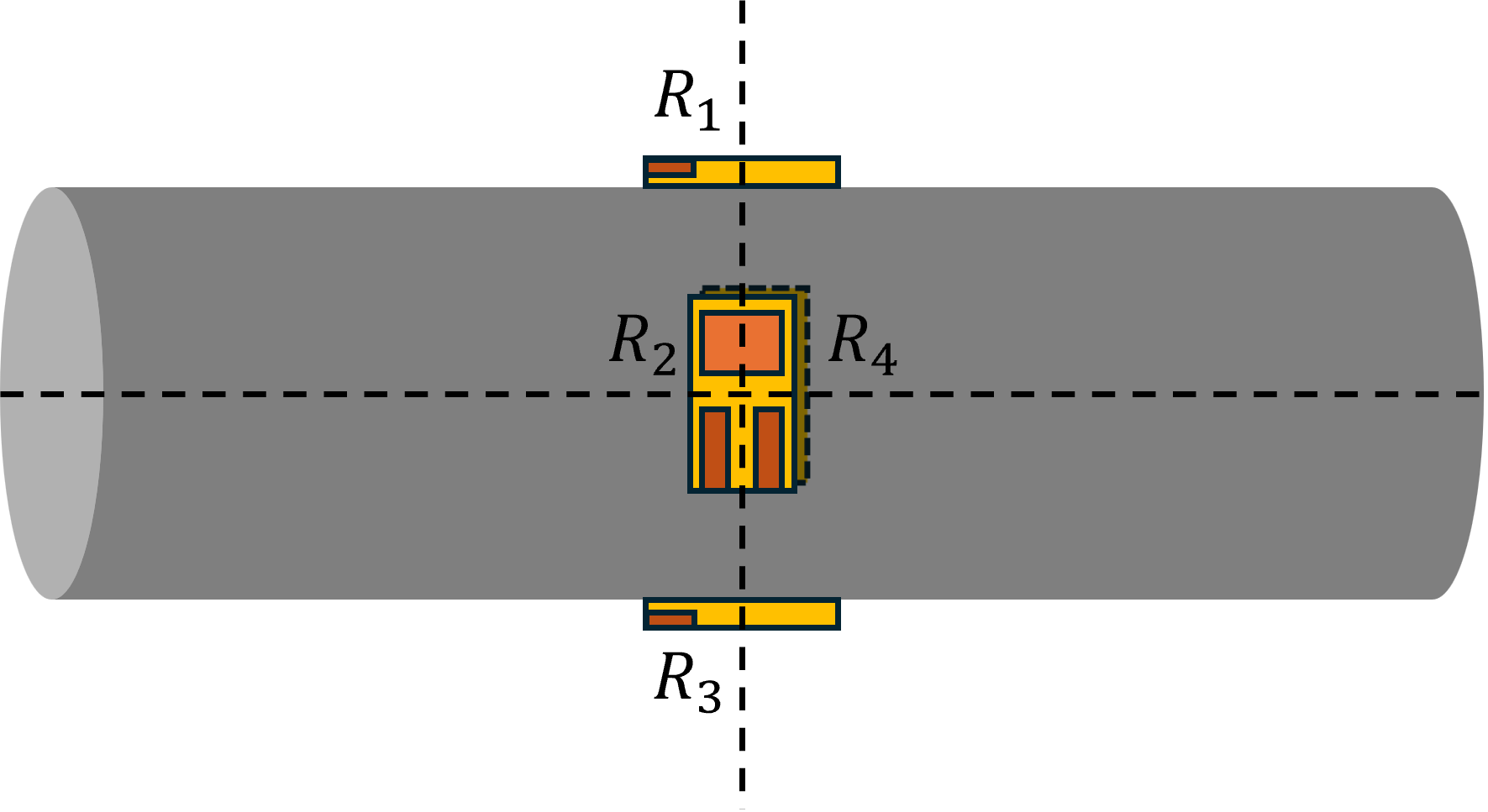
Strain gauges in a full-bridge configuration mounted on a bar.
In this configuration:
- Longitudinal Strain Measurement: Two strain gauges, \(R_1 R_3 \) are mounted along the axis of the bar. These gauges are positioned to measure the longitudinal strain, which occurs along the length of the bar.
- Lateral Strain Measurement: The other two strain gauges, \(R_2 R_4 \) are oriented in the lateral direction, perpendicular to the longitudinal axis. They are mounted along the circumference of the bar and are responsible for measuring the lateral strain.
All four strain gauges are aligned such that a common center line passes through each one, ensuring consistent and accurate strain measurement. This precise alignment and placement allow the full bridge circuit to effectively capture both longitudinal and lateral strains, providing a comprehensive analysis of the mechanical deformation experienced by the bar.
Strain Gauge Installation Techniques
The process of mounting strain gauges onto a metal surface involves several key steps to ensure accurate measurements. Firstly, the surface of the metal must be thoroughly cleaned to remove any contaminants such as oil, dirt, or oxidation. This is typically done using solvents and abrasive materials.
Once the surface is prepared, a high-quality adhesive is applied to the back of the strain gauge. Common adhesives include cyanoacrylate for quick bonding or epoxy for stronger, more durable bonds. The strain gauge is then carefully positioned on the cleaned metal surface, ensuring proper alignment.
After placement, pressure is applied to the gauge to ensure firm contact and eliminate any air bubbles. The adhesive must be allowed to cure according to the manufacturer's instructions. Curing times can vary from a few minutes to several hours, depending on the type of adhesive used. In some cases, heat may be applied to accelerate the curing process.
Proper mounting and curing are crucial to the performance of the strain gauge, as any movement or misalignment during this process can affect the accuracy of the strain measurements.
Experiment Results #
Conversion of Voltage to Strain for Strain Gauge Measurements
In the Split Hopkinson Pressure Bar (SHPB) experiment, strain gauges are typically placed on the input and output bars to measure the incident, reflected, and transmitted pulses during the test. These strain gauges produce voltage signals in response to the strain experienced by the bars.
Follow these steps to convert the output voltage data from the strain gauges to strain:
1. Calibration of Strain Gauges:
Each strain gauge has a specific gauge factor (GF). This is a sensitivity coefficient that relates the change in resistance (or voltage) to the strain experienced by the gauge. It is defined as:
\[ \text{GF} = \frac{\Delta R}{R_0 \cdot \varepsilon} \]
Where:
- \(\Delta R\) is the change in resistance of the gauge due to strain.
- \(R_0\) is the original resistance of the gauge.
- \(\varepsilon\) is the strain experienced by the gauge.
2. Measure Voltage Output:
During the experiment, strain gauges measure the strain experienced by the bars and convert it into voltage changes. Use a data acquisition system (DAQ) to record the voltage output from the strain gauges.
3. Convert Voltage to Strain:
Convert the voltage change to strain using the gauge factor and the applied excitation voltage. The relationship between the change in voltage (\(\Delta V\)) and the strain (\(\varepsilon\)) is given by:
\[ \varepsilon = \frac{\Delta V}{V_{\text{ex}} \cdot \text{GF}} \]
Where:
- \(V_{\text{ex}}\) is the excitation voltage applied to the strain gauge.
- \(\Delta V\) is the change in voltage output from the strain gauge.
Apply the formula to each recorded voltage output from the strain gauges. This will give you the strain experienced by the bar at the location of each gauge.
Further processing may be required to filter the data and remove any noise or high-frequency components that could interfere with your analysis.
Analyze the strain-time data to determine the mechanical properties of the specimen, such as stress-strain curves, strain rate, and other parameters.
Conversion of Output Voltage Data to Strain in SHPB Experiment
In the Split Hopkinson Pressure Bar (SHPB) experiment, strain gauges are typically placed on the input and output bars to measure the incident, reflected, and transmitted pulses during the test. These strain gauges produce voltage signals in response to the strain experienced by the bars. Converting the output voltage data from strain gauges to strain requires the use of several key parameters, including the amplifier gain, the gauge factor of the strain gauge, and the bridge factor of the strain gauge configuration.
1. Output Voltage Data: The strain gauges used in the SHPB experiment produce an output voltage, denoted as \( V_{\text{out}} \), in response to strain. This output voltage is a measure of the change in resistance of the strain gauge due to mechanical deformation.
2. Excitation Voltage: The strain gauges are typically connected in a Wheatstone bridge configuration, which is excited by a known voltage, denoted as \( V_{\text{excited}} \).
3. Amplifier Gain: The output from the Wheatstone bridge may be amplified using an amplifier. The gain, denoted as \( G \), of the amplifier influences the relationship between the actual output voltage and the measured output voltage.
4. Gauge Factor: The gauge factor, denoted as \( \text{G.F.} \), quantifies the sensitivity of the strain gauge to strain. It is a constant provided by the manufacturer that relates the change in resistance to the applied strain.
5. Bridge Factor: The bridge factor, denoted as \( \text{B.F.} \), accounts for the configuration of the strain gauges in the Wheatstone bridge. In a full bridge configuration, four strain gauges are typically connected in the bridge, and the bridge factor can vary depending on the arrangement of the gauges.
The formula to convert the output voltage data from the strain gauges to strain is:
\[ \frac{V_{\text{out}}}{V_{\text{excited}}} = \frac{\varepsilon \times G \times \text{G.F.} \times \text{B.F.}}{4} \]
This formula can be rearranged to solve for strain:
\[ \varepsilon = \left( \frac{V_{\text{out}}}{V_{\text{excited}}} \right) \times \left( \frac{4}{G \times \text{G.F.} \times \text{B.F.}} \right) \]
Bridge Factor Explanation
When using a full bridge configuration with alternating longitudinal and lateral strain gauges (long-lat-long-lat) in the Split-Hopkinson Pressure Bar (SHPB) experiment, the correct bridge factor (B.F.) can be determined based on the contributions of the longitudinal and lateral gauges and the Poisson's ratio (\(\mu\)) of the bar material.
Explanation: In a full bridge setup with alternating longitudinal and lateral gauges, each gauge measures a different strain: longitudinal gauges measure axial strain, while lateral gauges measure lateral strain (which is related to axial strain through Poisson's ratio).
The overall bridge factor is a weighted sum of the sensitivity of the four gauges. Since the lateral gauges respond to the Poisson's effect, their response must be adjusted according to the Poisson's ratio of the bar material.
The simplest formula for calculating the bridge factor in this configuration is:
\[ \text{B.F.} = 2 \times (1 + \mu) \]
Where:
- \( \text{B.F.} \) is the bridge factor for the full bridge configuration.
- \( \mu \) is the Poisson's ratio of the bar material.
This formula is derived from the contributions of the two longitudinal and two lateral gauges in the bridge, accounting for the effect of Poisson's ratio on the lateral gauges.
Therefore, using the formula \( \text{B.F.} = 2 \times (1 + \mu) \) for calculating the bridge factor is the correct theory for the full bridge long-lat-long-lat configuration.
Bridge Factor Explanation for Different Configurations
When all the strain gauges in the Split-Hopkinson Pressure Bar (SHPB) experiment are oriented in the longitudinal direction, the calculation of the bridge factor (B.F.) depends on whether the gauges are configured in a full bridge or a half bridge setup.
1. Full Bridge Configuration (Longitudinal Gauges):
In a full bridge configuration with all gauges oriented in the longitudinal direction, the bridge factor (B.F.) is equal to the total number of strain gauges in the bridge. Since all the gauges are aligned in the same orientation, their individual contributions are directly added.
\[ \text{B.F.} = \text{number of gauges in the bridge} = 4 \]
Therefore, in a full bridge configuration with all longitudinal gauges, the bridge factor is typically equal to 4.
2. Half Bridge Configuration (Longitudinal Gauges):
In a half bridge configuration with all gauges oriented in the longitudinal direction, there are two active strain gauges in the circuit, and the other two resistors in the Wheatstone bridge are reference resistors.
\[ \text{B.F.} = \text{number of active gauges in the bridge} = 2 \]
Therefore, in a half bridge configuration with all longitudinal gauges, the bridge factor is equal to 2.
3. Strain Gauge Rosette (Longitudinal-Lateral Configuration):
A strain gauge rosette consists of gauges oriented in different directions, typically in a long-lat configuration (longitudinal and lateral). In a half bridge setup with a strain gauge rosette, two strain gauges are oriented differently and connected in the bridge circuit, which creates a half bridge configuration.
\[ \text{B.F.} = \text{number of active gauges in the rosette} = 2 \]
Therefore, in a strain gauge rosette with a long-lat configuration used in a half bridge setup, the bridge factor is equal to 2.
4. Single or QuarterBridge Configuration:
In a quarter bridge configuration, there is one active strain gauge and three reference resistors. This setup is simpler and provides less sensitivity compared to the half or full bridge configurations.
\[ \text{B.F.} = \text{number of active gauges in the bridge} = 1 \]
Therefore, in a quarter or single bridge configuration, the bridge factor is equal to 1.
Knowing the bridge factor is crucial for accurately converting output voltage data from the strain gauges to strain in the SHPB experiment.
Plotting of Experimental Results
- Raw data, typically in the form of voltage-time measurements, cropped and combined to obtained incident, reflected, and transmitted bars voltages, is collected during the experiment.
- To reduce noise and extract meaningful information, a Savitzky-Golay filter is applied to the raw voltage-time data. This filtering process smooths out fluctuations and enhances the accuracy of subsequent calculations.
- The filtered voltage data is converted to strain using a predefined conversion relation. This step involves multiplying the voltage measurements by a conversion factor to obtain strain values.
- Based on the strain data, particle velocities at the specimen/input-bar and specimen/output-bar interfaces are calculated using the bar wave speed and differences in strain between incident, reflected, and transmitted waves.
- The mean axial strain rate in the specimen is computed from the differences in particle velocities normalized by the initial length of the specimen.
- The strain rate data is integrated over time to obtain nominal strain using numerical integration techniques.
- Nominal stress in the specimen is calculated using the measured voltage data, material properties, and cross-sectional areas of the bars.
- Finally, true strain is computed from the nominal strain, and true stress is obtained by correcting the nominal stress using the true strain.
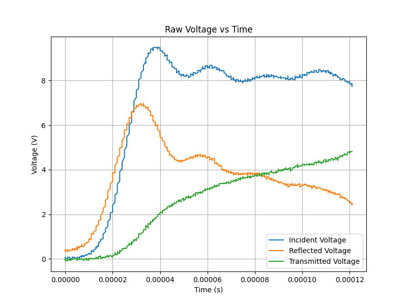
Raw Amplified Voltage-Time Data (Cropped and combined)
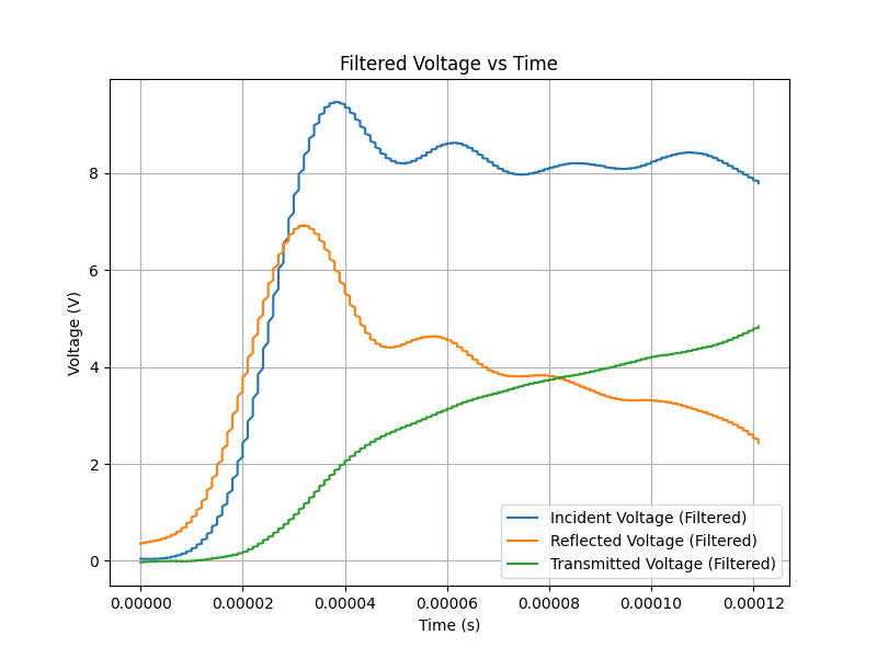
Filtered Amplified Voltage-Time Data (Savitzky-Golay filter)
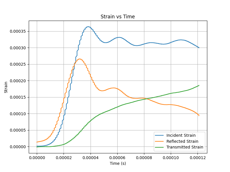
Strain-Time Data (voltage data converted to strain)
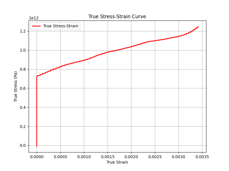
True Stress-Strain
Analysis of Data #
Code Explanation and Pointers
Importing Libraries: The code imports necessary libraries such as Pandas for data manipulation, NumPy for numerical computations, Matplotlib for plotting, and functions from SciPy for signal filtering and numerical integration.
Input Parameters: Initial values for various physical parameters like Young's modulus, density, initial length, and cross-sectional areas of bars and specimen are provided.
Reading Data: The code reads experimental data from a CSV or Excel file depending on the specified file type. It extracts time, incident voltage, reflected voltage, and transmitted voltage data from the file.
Filtering Data: Savitzky-Golay filter is applied to smooth out noise in the voltage data.
Calculating Strain and Strain Rates: The filtered voltage data is converted into strain using a provided relation. Then, particle velocities at specimen/bar interfaces are calculated, followed by mean axial strain rate in the specimen.
Integrating Strain Rate: The mean axial strain rate is integrated over time to obtain nominal strain using cumulative trapezoidal integration.
Calculating Stress: Nominal stress in the specimen is calculated using the transmitted voltage data and physical parameters.
Calculating True Strain and True Stress: True strain is calculated using logarithmic strain transformation, and true stress is calculated based on nominal stress and true strain.
Plotting: The code then plots various data and results. It first plots the raw voltage data over time, then the filtered voltage data, strain data, stress-strain curve (nominal), and true stress-strain curve.
Analysis Code Instructions
-
1. Install Dependencies:
Make sure you have Python installed on your system. You can install the required Python packages by running the following command:
pip install -r requirements.txt -
2. Prepare Experimental Data:
- Ensure that your experimental data is stored in a CSV or Excel file.
- The file should contain columns for "Time", "Incident", "Reflected", and "Transmitted" voltages.
- Voltage values should be in volts (V)
- Specify the file name in the Python script (analysis.py) using the filename variable. For example:
filename = "path/to/your/data_file.csv" -
3. Customize Input Parameters:
- Open the Python script (analysis.py) in a text editor.
- Update the input parameters according to your experiment setup. Parameters such as Young's modulus, density, initial length, and cross-sectional areas should be adjusted based on your experimental conditions.
-
4. Run the Script:
Run the script using the following command:
python analysis.py -
5. View Plots and Analyze Results:
- After running the script, view the generated plots to analyze the results.
- The script will generate plots for filtered voltage data, strain data, stress-strain curve, and true stress-strain curve.
Links to SHPB Analysis Code
Code on GitHubReferences #
- Ramesh, K.T. (2008). High Rates and Impact Experiments. In: Sharpe, W. (eds) Springer Handbook of Experimental Solid Mechanics. Springer Handbooks. Springer, Boston, MA. DOI: 10.1007/978-0-387-30877-7_33
- Kolsky, H. (1963). Stress Waves in Solids. United Kingdom: Dover Publications.
- Chen, W. W., & Song, B. (2011). Split Hopkinson (Kolsky) Bar Design, Testing and Applications. Springer.
- Lifshitz, J. M., & Leber, H. (1994). Data Processing in the Split Hopkinson Pressure Bar Tests. International Journal of Impact Engineering, 15(6), 723-733. Elsevier Science Ltd.
- Johnson, W. (1972). Impact strength of materials, Edward Arnold, London.
